ARTICLE: Dust Grain-Size Distributions and Extinction in the Milky Way, Large Magellanic Cloud, and Small Magellanic Cloud

In Journal Club, Journal Club 2011 on February 19, 2011 at 7:50 pm

Read the paper by Weingartner & Draine (2001)

Summary by Max Moe and Katherine Rosenfeld.
Click here to download a pdf version of the class handout.

Abstract:

We construct size distributions for carbonaceous and silicate grain populations in different regimes for the Milky Way, LMC, and SMC. The size distributions include very small carbonaceous grains (including polycyclic aromatic hydrocarbon molecules) to account for the observed infrared and microwave emission from the diffuse interstellar medium. Our distributions reproduce the observed extinction of starlight, which varies depending on the interstellar environment through which the light travels. As shown by Cardelli, Clayton, and Mathias in 1989, these variations can be roughly parameterized by the ratio of visual extinction to reddening, $R_v$ . We adopt a fairly simple functional form for the size distributions, characterized by several parameters. We tabulate these parameters for various combinations of values for $R_v$ and $b_c$ , the Carbon abundance of very small grains. We also find size distributions for the line to HD 210121 and for sigh lines in the LMC and SMC. For several size distributions, we evaluate the albedo and scattering asymmetry parameter and present model extinction curves extending beyond the Lyman limit.

Background and Motivation:

The size of dust grains along with composition and geometry will determine the extinction of light as it travels through a dust cloud in the interstellar medium. The intensity goes as:
$I(\lambda) = I_0(\lambda) e^{-\tau(\lambda)}$
and so the extinction goes as:
$A(\lambda) = -2.5 \log I/I_0 \approx -1.086 \ln e^{-\tau(\lambda)} = 1.086 \tau(\lambda)$ .
The optical depth, $\tau$ , is related to to the size of the particles via their cross section. Previous to this work, other works (Mathis, Rumpl, & Nordsiek) had fit observed interstellar extinction using distributions of particle sizes well fit by a power law with index of about -3.5. Since that work in 1977, further observations of the diffuse interstellar medium suggested the existence of population of dust grains smaller than 50 angstroms. Furthermore, the lack of a 10 micron silicate feature suggested that this population should be largely composed of non-silicate grains and specific emission features were identified with carbonaceous compositions, specifically polycyclic aromatic hydrocarbons (PAHs). This paper tried to fit the extinctions that would result from a large small and large(er) grain population to reproduce the observed extinctions along various lines of sight.

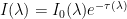
Figure 4 from Mathis, Nordsieck, and Rumpl (1977) showing the modeled optical depth (dots and triangles) and observed optical depth (solid one). The dashed line is the contribution of graphite to the extinction.

Considering different lines of sight is important because extinction varies on the environment that the light is passing though. The ratio of extinction in the V band (e.g. visual extinction) to reddening, 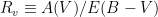$R_v \equiv A(V)/E(B-V)$ , had been previously shown to parametrize this extinction. Therefore the model featured in this paper used this parameter as a proxy of interstellar environment.

The Calculation

Grain size distribution:

Lacking a theory for the distribution of interstellar grain sizes, the authors used a simple functional form that had control over some maximum grain size, the steepness of this size cutoff, and the slope of the distribution of grains below the cutoff. They included two main species of grains, silicate and carbonaceous, where both had the same functional form but with an additional small grain population for the carbonaceous grains. They modeled this population using two log-normal size distributions centered at 3.5 and 30 $\AA$ to explain observed dust emission in the microwave and IR bands as well as the 750 and 2175 $\AA$ extinction features. See equations (2) – (6) to see the equations written out in full. Taking both grain species together leaves 11 parameters for fitting: 5 for silicon and 6 for cabonaceous grains. The extra parameter is the Carbon abundance, $b_c$, which is a proxy for the contribution of the small grains.

Modeling the extinction:

Given a grain-size distribution and its composition, the authors then calculate the extinction at a specific wavelength:

$A(\lambda) = (2.5 \pi \log e) \int d \ln a \frac{d N_{gr} (a)}{da} a^3 Q_{ext}(a,\lambda)$ .

$N_{gr}(a)$ is the column density of grains with size less than a and is computed from the grain size distribution. The hard physics comes from teh extinction efficiency factor, $Q_{ext}$ which is generally a function of size, geometry, composition, and wavelength. The authors assume a simple spherical geometry and grains of a single composition – no ice mantles, mixed species, or conglomerated grains (see figure below). The calculation is done using a Mie scattering code that requires the dialectric function of the material (also a function of size, composition, and wavelength). The Mie scattering theory also considred albedo and asymmetry effects.

Albedo and asymmetry for a number of size distributions. Figure 15 from Weingartner and Draine.

For the silicate grains the authors use results from laboratory measurement of crystalline olivine smoothed over to remove a feature that is not observed. The carbonaceous grains are assumed to have a compositional distributiion as well where the smallest grains are PAH molecule, largest are graphite, and in between are some mixture. Since we don’t really know what the PAHs are exactly, the dialectric function is derived from astronomical observations.

Example extinction coefficients calculated from Mie Theory. From pg 58 of Voshchinnikov's "Optics of Cosmic Dust I"

Putting all of this together, the authors generate extinction curves for a given $R_v$ and $b_c$ and fit by minimizing one or two error functions. The first (case B) considers the error in the modeled and observed extinction. The other (case A) includes abundance and depletion values calculated from solar neighborhood values. The motivation for Case A is to avoid fits for high $R_v$ that reduce the grain volume past astrophysical intuition. Click here for a graphical sketch of the fitting process.

Grain-size distributions for Rv = 3.1. Figure 2 from Weingartner & Draine.

Model extinction curve optimized to fit the observed curve. Figure 8 from Weingartner & Draine.

Results and Discussion:

The paper considers dust in the Milky Way and towards HD 210121, the LMC and the SMC. With a small value of $R_v$ , features weaker than parametrized by $R_v$ , and a strong UV rise, HD 210121 was a test of the model. The authors were able to find grain-size distributions for $b_c = [0.0, 4.0]$ and conclude that their grain model dealt well with thin line of sight. Table 2 contains the fitted parameters and the silicate grain volume for all cases exceeds that of the solar neighborhood. In class we discussed how this parameter probes star formation history since silicates are produced in supernovae and not in the winds of hot AGB stars like carbonaceous grains. Next they considered the lines of sight towards the metal poor LMC and SMC – a useful test of the model applied to extragalactic sources.

Direct or in situ measurement of ISM grain size distributions are rare and difficult to make. High altitude airplanes can collect inter-planetary dust (IPD) including GEMS grains (glass with embedded metal and sulfides) that, while much larger than the dust considered in this paper, are very primitive grains. NASA’s Stardust mission captured cometary particles and successfully delivered the payload back to Earth.

An interplanetary dust particle. From http://www.astro.washington.edu/users/brownlee/.

A GEMS particle. Image from http://stardust.jpl.nasa.gov.

The Ulysses and Galileo spacecraft also made in situ measurement of the local interstellar medium by measuring the impact of interstellar grains. The model presented in this paper appears to underestimate the number of large particles while overestimating the number of small particles (Frisch et al, 1999). Size-sorting and segregation are listed as possible causes of the disagreement.

Mass distribution of grains in the local ISM from spacecraft measurements and the presented models. Figure 24 from Weingartner & Draine.

While there are a number of acknowledged caveats assumptions in this relatively simple model, the model appears consistent with observations. Improvements that could be added to the model include adding a coating layer to the grains to reproduce the 3.4 micron feature or weak inter-stellar bands. Regardless, this simple model is sufficient and consistent in reproducing extinction curves so that errors and deviations in depletion, metallicities, dielectric constants, etc. are somewhat negligible. In addition, for a given environment the grain size distribution appears to vary. This suggests that small grains come together to form large grains especially in dense clouds. Similarly, collisions in shock waves can shatter the large grains and replenish the small grain population. Lastly, the cutoff in the size distribution is limited by the timescales of coagulation, shattering, accretion, and erosion along with the proportion between PAH molecules (small grains) and graphite (large grains).

One caveat is that while this paper assume spherical dust grains, real dust is more composite, fluffy, and amorphous. Furthermore, the derived grain-size distribution is disparate from dust in the local ISM. Interstellar dust passing through our solar system has a steeper slope dominated by larger grains as well as a larger cut-off in maximum size. Fundamentally, the dielectric functions used are not accurate for silicates and graphites, and especially so for PAHs. Lastly, degeneracies remain in some fitting parameters (e.g. the carbon grain-size slope at small sizes vs. $b_c$ ) so there parameters must be constrained from other observations.

For more information:

Heidelberg Cosmic Dust Group
Voshchinnikov’s Optics of Cosmic Dust I

▶ No Responses

Harvard Astronomy 201b

ISM and Star Formation