Wide-Field Near-Infrared Imaging of the L1551 Dark Cloud by Masahiko Hayashi and Tae-Soo Pyo
Observations of CO in L1551 – Evidence for stellar wind driven shocks by Ronald L. Snell, Robert B. Loren & Richard L. Plambeck
Multiple Bipolar Molecular Outflows from the L1551 IRS5 Protostellar System by Po-Feng Wu, Shigehisa Takakuwa, and Jeremy Lim
Summary by Fernando Becerra, Lauren Woolsey, and Walker Lu
Introduction
Young Stellar Objects and Outflows
In the early stages of star formation, Young Stellar Objects (YSOs) produce outflows that perturb the surrounding medium, including their parental gas cloud. The current picture of star formation indicates that once gravity has overcome pressure support, a central protostar is formed surrounded by an infalling and self-supported gas disk. In this context outflows are powered by the release of gravitational potential energy liberated by matter accreting onto the protostar. Outflows are highly energetic and often spatially extended phenomena, and are observable over a wide range of wavelengths from x-ray to the radio. Early studies of molecular outflows (predominantly traced by CO emission lines, e.g. Snell et al. 1980, see below) have shown that most of their momentum is deposited in the surrounding medium and so provide a mass loss history of the protostar. In contrast, the optical and near-infrared (NIR) emission trace active hot shocked gas in the flow.
Interactions with the surrounding medium: Herbig-Haro objects, bow shocks and knots
When outflows interact with the medium surrounding a protostar, emission can often be produced. One example of this is emission from Herbig-Haro (HH) objects, which can be defined as “small nebulae in star-forming regions as manifestations of outflow activity from newborn stars”. The most common pictures show a HH object as a well-collimated jet ending in a symmetric bow shock. Bow shocks are regions where the jet accelerates the ambient material. The shock strength should be greatest at the apex of the bow, where the shock is normal to the outflow, and should decline in the wings, where the shocks become increasingly oblique. Another interesting feature we can distinguish are knots. Their origin is still unknown but a few theories have been developed over the years. They can formed due to the protostar producing bursts of emission periodically in time, or producing emission of varying intensity. They can also form due to interactions between the jet and the surrounding Interstellar Medium (ISM), or due to different regions of the jet having different velocities.
An exceptional case: The L1551 region
The L1551 system is an example of a region in which multiple protostars exhibiting outflows are seen, along with several HH objects and knots. This system has been catalogued for over fifty years (Lyons 1962), but ongoing studies of the star formation and dynamical processes continue to the present day (e.g. Hayashi and Pyo 2009; Wu et al. 2009). L1551 is a dark cloud with a diameter of ~20′ (~1 pc) located at the south end of the Taurus molecular cloud complex. The dark cloud is associated with many young stellar objects. These YSOs show various outflow activities and characteristics such as optical and radio jets, Herbig-Haro objects, molecular outflows, and infrared reflection nebulae. We will start by giving a broad view of the region based on Hayashi and Pyo 2009, and then we will focus on a subregion called L1551 IRS 5 following Snell et al. 1980 and Wu et al. 2009.
Paper I: An overview of the L1551 Region (Hayashi and Pyo 2009)
The L1551 region is very rich in YSOs, outflows and their interaction with the ISM. The most prominent of the YSOs in this region are HL Tau, XZ Tau, LkHα 358, HH 30, L1551 NE, and L1551 IRS 5 (see Fig. 1), arrayed roughly north to south and concentrated in the densest part (diameter ~10′) of the cloud. The authors based their study on observations using two narrowband filters [Fe II] ( = 1.6444 μm,
  = 0.026 μm),
  ( = 2.116 μm, = 0.021 μm) and two broad-band filters:
  ( = 1.64 μm, = 0.28 μm)
  ( = 2.14 μm, = 0.31 μm). The choice of [Fe II] and is motivated by previous studies suggesting that the [Fe II] line has higher velocity than the , and thus arises in jet ejecta directly accelerated near the central object, while emission may originate in shocked regions. In the particular case of bow shocks, regions of higher excitation near the apex are traced by [Fe II], while is preferentially found along bow wings. The broadband filters were chosen for comparison with NIR narrowband filters and comparison with previous studies. The total sky coverage was 168 arcmin2, focused on 4 regions of the densest part of the L1551 dark cloud, including HL/XZ Tau, HH30, L1551 IRS5, some HH objects to the west, L1551 NE, and part of HH 262 (see Fig. 1).
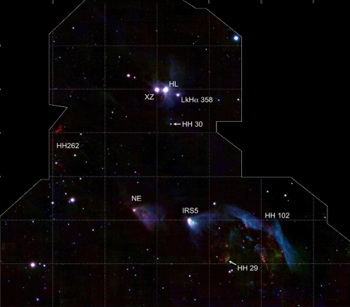
Figure 1: An overview of L1551 (Figure 1 of Hayashi and Pyo 2009)
HL/XZ Region
Some of the features the authors identify in this region are:
- A faint [Fe II] jet emanating from HL Tau to its northeast and southwest. The emission is hard to identify in the northeast part, but significant emission blobs are detected in the southwest part (denoted “H2 jet” in Fig. 2)
- A diffuse feature is also distinguished to the north-northeast of XZ Tau, which may be related to the outflow from one member of the XZ Tau binary.
- A continuum arc from HL Tau to the north and then bending to the east (“cont arc” in Fig. 2) is also identified. This arc may be a dust density discontinuity where enhanced scattering is observed. Although it is not clear if this arc is related to activities at HL Tau or XZ Tau.
- Another arc feature to the south from HL Tau curving to the southeast can be identified. Two features are located in the arc and indicated by arrows in Fig. 2. This may be shocked regions in the density discontinuity.
- Other features can be distinguished: “A” (interpreted as a limb-brightened edge of the XZ Tau counter-outflow) and “B”, “C”, “a” (blobs driven by the LkH
 358 outflow and interacting with the southern outflow bubble of XZ Tau).
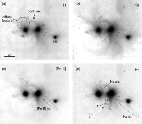
Figure 2: HL/XZ Region (Figure 2 of Hayashi and Pyo 2009)
HH 30 Region
HH 30 is a Herbig-Haro (HH) object including its central star, which is embedded in an almost edge-on flared disk. Although this object doesn’t have clear signs of large-scale [Fe II] or emission (see Fig. 3), a spectacular jet was detected in the [S II] emission line in previous studies. Despite that, the authors identify two faint small-scale features based on the [Fe II] frame: one to the northeast (corresponding to the brightest part of the [S II] jet) and one to the south-southeast (corresponding to a reflection nebula)
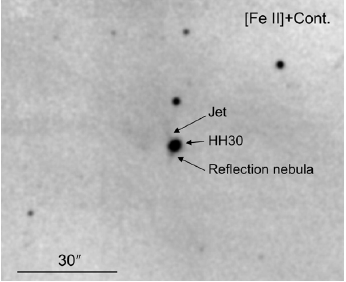
Figure 3: HH 30 Region (Figure 3 of Hayashi and Pyo 2009)
L1551 NE
L1551 NE is a deeply embedded object associated with a fan-shaped infrared reflection nebula opening toward the west-southwest seen in the broad-band Ks continuum emission. It has an opening angle of  . The most important features in this region are:
- A needle-like feature connecting L1551 NE and HP2 is distinguished from the continuum-substracted [Fe II] image, associated with an [Fe II] jet emanating from L1551 NE.
- A diffuse red patch at the southwest end of the nebula (denoted as HP1) is dominated by emission
- Five isolated compact features are detected in the far-side reflection nebula: HP3 and HP3E ([Fe II] emission), HP4 (both [Fe II] and emission) and HP5 and HP6 ( emission). All of them are aligned on a straight line that is extrapolated from the jet connecting NE and HP2, naturally assigned to features on the counter-jet.
- Comparing this data to previous observations in [S II] and radio we can deduce radial velocities of 160-190 km/s for HP2, and 140-190 km/s for HP4 and HP5. With radial velocities in the range 100-130 km/s for these knots, the inclination of the jet axis is estimated to be
 –.
–.
L1551 IRS-5
L1551 IRS 5 is a protostellar binary system with a spectacular molecular outflow (Snell et al. 1980; see below) and a pair of jets emanating from each of the binary protostars. A conspicuous fan-shaped infrared reflection nebula is seen in Fig. 4, widening from IRS 5 toward the southwest. At the center of this nebula, the two [Fe II] jets appear as two filaments elongated from IRS 5 to its west-southwest; the northern jet is the brighter of the two. Knots A, B and C located farther west and west-southwest of PHK3 (associated with line emission) have significant [Fe II] emission.
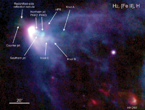
Figure 4: A close-up of IRS-5 (Figure 5 of Hayashi and Pyo 2009)
A counter-jet only seen in the [Fe II] frame can be distinguished to the northeast of IRS 5. Considering its good alignment with the northern jet, it can be interpreted as the receding part of the jet. Based on brightness comparison between the both jets, and transforming H-band extinction to visual extinction the authors deduce a total visual extinction of Av=20-30 mag. Besides the counter-jet, the authors also detect the northern and southern edge of the reflection nebula that delineate the receding-side outflow cone of IRS5.
A brief summary of the HH objects detected in the IRS5 region:
- HH29: Consistent with a bow shock, its [Fe II] emission features are compact, while the emission is diffuse. Both emissions are relatively separate.
- HH260: Consisted with a bow shock with compact [Fe II] emission knot located at the apex of a parabolic emission feature.
- HP7: Its [Fe II] and emission suggest it is also a bow shock driven by an outflow either from L1551 IRS5 or NE.
- HH264: It is a prominent emission loop located in the overlapping molecular outflow lobes of L1551 IRS5 and NE. Its velocity gradients are consistent with the slower material surrounding a high-velocity (~ -200 km/s in radial velocity) wind axis from L1551 IRS 5 (or that from L1551 NE)
- HH 102: Loop feature dominated by emission (and no [Fe II] emission) similar to HH264. Considering that the major axes of the two elliptical features are consisted with extrapolated axis of the HL Tau jet, it is suggested that they might be holes with wakes on L1551 IRS5 and/or NE outflow lobe(s) that were bored by the collimated flow from HL Tau.
Comparison of Observations
Near-infrared [Fe II] and emission show different spatial distributions in most of the objects analyzed here. On one hand the [Fe II] emission is confined in narrow jets or relatively compact knots. On the other hand, the emission is generally diffuse or extended compared with the [Fe II] emission, with none of the features showing the well collimated morphology as seen in [Fe II].
These differences can be understood based on the conditions that produce different combinations of [Fe II] and emission:
- Case of spatially associated [Fe II] and emissions: Generally requires fast dissociative J shocks (Hollenbach & McKee 1989; Smith 1994; Reipurth et al. 2000).
- Case of a strong emission without detectable [Fe II] emission: Better explained by non-dissociative C shocks
The interpretation of differences in [Fe II] and emission as a result of distinct types shocks is supported by observational evidence showing that the [Fe II] emission usually has a much higher radial velocity than the emission. In the case of HH 29, HH 260 and HP 7 the [Fe II] emission arises in the bow tips where the shock velocity is fast (~50 km/s) and dissociative whereas emission occurs along the trailing edges where the shock is slower (~20 km/s)
Paper II: Landmark Observations of Snell et al. 1980
One of the original papers in the study of L1551 was written by Snell, Loren and Plambeck (1980). In this paper, the authors use 12CO to map what they find to be a double-lobed structure extending from the infrared source IRS-5 (see Figures 1, 4). This system is also associated with several Herbig-Haro objects, which are small dense patches that are created in the first few thousands of years after a star is formed. This star is consistent with a B star reddened by 20 magnitudes of dust extinction along the line of sight, through a distance of 160 pc (Snell 1979). By studying these outflows, we are able to better understand the evolution of YSOs.
Observations
Snell et al. (1980) made their observations using the 4.9 meter antenna at Millimeter Wave Observatory in Texas. Specifically, they considered the J = 1-0 and J = 2-1 transitions of  CO and
  CO. Additionally, they made J = 1-0 observations with the NRAO 11 meter antenna. They found asymmetries in the spectral lines, shown below in Figure 5. To the northeast of IRS-5, the high-velocity side of the line has a broad feature, and the southwest of IRS-5 presents a similar broad feature on the low-velocity side of the spectral line. No such features were found to the NW, SE, or in the central position of IRS-5.
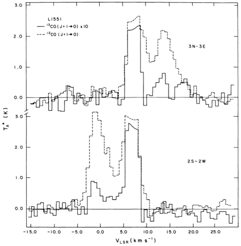
Figure 5: 12CO and 13CO 1-0 transition lines; top is NE of central source, bottom is SW of source (Figure 4 of Snell et al. 1980)
The J = 2-1 CO transition is enhanced relative to the J = 1-0 transition of CO, suggesting that the CO emission is not optically thick. If the emission was optically thick, the J = 1-0 line would be the expected dominant transition as it is a lower level transition. The observations also suggest an excitation temperature for the 2-1 transition of T ~ 8-35 K. This would only relate to the gas temperature if the environment is in local thermal equilibrium, but it does set a rough minimum temperature. The CO emission for the 1-0 transition is roughly 40 times weaker than the same transition for CO, which further suggests both isotopes are optically thin in this region (if the CO is already optically thin, the weaker transition means CO is even more so). The geometry of the asymmetries in the line profiles seen to the NE and SW combined with the distance to L1551 suggest lobes that extend out 0.5 pc in both directions.
Interpretations
Column density
The authors make a rough estimate of the column density of the gas in these broad velocity features by making the following assumptions:
- the CO emission observed is optically thin
- the excitation temperature is 15 K
- the ratio of CO to H2 is a constant

With these assumptions, the authors find a column density of  . This is much lower than the region’s extinction measurement of
  20 magnitudes by Snell (1979), as the outflow is sweeping out material around the star(s).
Stellar wind and bow shocks
The model of the wind that Snell et al. (1980) suggest is a bimodal wind that sweeps out material in two “bubble-like” lobes, creating a dense shell and possible ionization front that shocks the gas (More on shocks). The physical proximity of the Herbig-Haro (HH) objects in the southwest lobe coming from IRS-5 suggests a causal relationship. Previous work found that the optical spectra of the HH objects resemble spectra expected of shocked gas (Dopita 1978; Raymond 1979).
There is evidence that the CO lobes are the result of a strong stellar wind, the authors clarify this with the schematic shown in Figure 6. They suggest that the wind is creating a bow shock and a shell of swept-up material (More on outflows in star-forming regions). The broad velocity features on the CO emission line wings reach up to 15 km/s, suggesting the shell is moving out at that speed. The Herbig-Haro objects HH29 and HH102 have radial velocities of approximately 50 km/s in the same direction as the SW lobe is expanding (Strom, Grasdalen and Strom 1974). Additionally, Cudworth and Herbig (1979) measured the transverse velocities of HH28 and HH29, and found that the objects were moving at a speed of 150 to 170 km/s away from IRS-5. To have reached these velocities, the HH objects must have been accelerated, most likely by a strong stellar wind at speeds above 200 km/s. The bimodal outflow suggests a thick accretion disk around the young star.
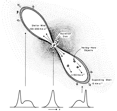
Figure 6: Schematic drawing of stellar outflow (Figure 5 of Snell et al. 1980)
Mass-loss rate
The average density in the region away from the central core is  (Snell 1979), so the extent and density of the shell implies a swept-up mass of 0.3 to 0.7 solar masses. With the measured velocity of ~15 km/s assumed to be constant during the lifetime of the shell and at the measured distance of 0.5 pc from the star, the shell was created 30,000 years ago. With this age, the authors determined a mass loss using the lower end of the assumed swept-up mass and the observed volume of the shell. They found a mass-loss rate of
  , which can be compared to other stars using a chart like that shown in Figure 7. This is not meant to present constraints on the processes that produce the mass loss in the IRS-5 system, but rather to simply provide context for the stellar wind observed. The low-mass main sequence star(s) that will eventually arise from the IRS-5 system will be characterized by much lower mass loss rates, and studies of mass loss rates from other YSOs suggest that this source is at the high end of the range of expected rates.
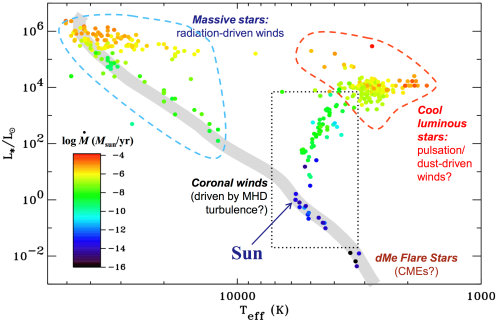
Figure 7: A representative plot of the different types of stellar wind, presented by Steve Cranmer in lectures for Ay201a, Fall 2012
Snell et al. (1980) suggest observational tests of this wind-driven shock model:
- H2 emission from directly behind the shock
- FIR emission from dust swept up in the shell; this is a possibly significant source of cooling
- radio emission from the ionized gas in the wind itself near to IRS-5 with the VLA or similar; an upper limit of 21 mJy at 6 cm for this region was determined by Gilmore (1978), which suggests the wind is completely ionized
The results of some newer observations that support this wind model are presented in the following section.
Paper III: A new look at IRS-5 by Wu et al. 2009
Wu et al. (2009) focus on the outflows in L1551 IRS5, the same region studied by Snell et al. (1980), but at a higher angular resolution (~3 arcsec; <1000 AU) and much smaller field of view (~1 arcmin; ~0.05 pc or 10,000 AU). Using the sub-millimeter array (SMA) right after it was formally dedicated, the authors detected CO(2-1) line and millimeter continuum in this low-mass star formation system. The mm continuum, which comes mostly from thermal dust emission, is used to estimate the dust mass. The CO(2-1) spectral line is used to trace the outflows around the binary or triple protostellar system at the center, revealing complex kinematics that suggest the presence of three possible bipolar outflows. The authors construct a cone-shaped outflow cavity model to explain the X-shaped component, and a precessing outflow or a winding outflow due to orbital motion model to explain the S-shaped component. The third component, the compact central one, is interpreted as newly entrained material by high-velocity jets.
Important concepts
There are several concepts related to radio interferometry that merit some discussion:
1. Extended emission filtered out by the interferometer
This is the well-known ‘missing flux problem’ unique in interferometry. There is a maximum scale over which structure cannot be detected by an interferometer, and this scale is set by the minimum projected baseline (i.e. projected distance between a pair of antennas) in the array. In the channel maps (Fig. 3 of Wu et al. 2009), there is a big gap between 5.8 km/s and 7.1 km/s. It does not indicate that there is no CO gas at these velocities, but rather is the result of very extended and homogenous CO distribution which is unfortunately filtered out. This effect applies to all channels.
2. Visibility vs. image
The data directly obtained from the interferometers are called visibility data, in which the amplitude and phase are stored for each baseline. The amplitude, as it literally means, measures the flux; and the phase derives the relative location with respect to the phase center (a reference position on the antenna). We need to convolve the visibility data with a point spreading function, also called ‘dirty beam’, to get the image we need. Mathematically, visibility and image are related through a Fourier transform. For more information, see this online course.
3. Channel maps and P-V diagram
In radio observations, velocity of spectral lines plays an important role by providing kinematic information inside ISM. Normally, the radio data has (at least) three dimensions, two in spatial (e.g. R.A. and Decl.) and one in frequency or velocity. Velocity itself can be used to identity outflows, turbulence or infall by the analysis of line profile, or it can be combined with spatial distribution of emission, if the spatial resolution allowed as in this paper, in the form of channel maps or P-V diagram, to show the three-dimensional structure. In terms of outflows, we expect to see gas at velocities much different from the systematic velocity, and a symmetric pattern both in red- and blue-shifted sides will be even more persuasive. For the efforts in visualizing the 3-d datacube in a fancier way, see this astrobite.
The classical image of low-mass star formation
Fig. 8 shows a diagram of a simplified four-step model of star formation (Fig. 7 of Shu et al. 1987). First, the dense gas collapses to form a core; second, a disk forms because of conservation of angular momentum; third, a pair of outflows emerge along the rotational axis; finally, a stellar system comes into place. During this process, bipolar outflows are naturally formed when the wind breaks through surrounding gas. Therefore, bipolar outflows are useful tools to indirectly probe the properties of protostellar systems.
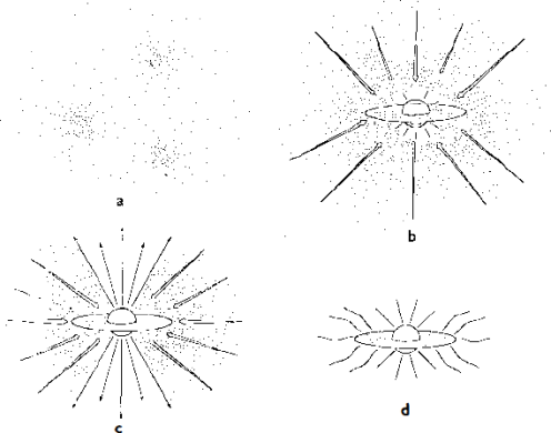
Figure 8: The formation of a low-mass star (see Shu et al. 1987)
Protostar candidates in L1551 IRS5
Two protostellar components as well as their own ionized jets and circumstellar disks have been found in this source. In addition, Lim & Takakuwa (2006) found a third protostellar candidate, as seen in Fig. 9. In this paper the authors investigated the possible connection between these protostars and the outflows.
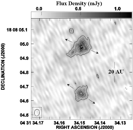
Figure 9: Two 7mm continuum peaks in the north and south represent the binary system in IRS 5. Arrows show the direction of jets from each of the protostars. A third protostellar candidate is found close to the northern protostar, marked by a white cross. (see Lim and Takakuwa 2006)
Three outflow components
Based on CO(2-1) emission, the authors found three distinct structures. Here the identification was not only based on morphology, but also on the velocity (see Fig. 5 and Fig. 9 of Wu et al. 2009). In other words, it is based on information in the 3-d datacube, as shown in 3 dimensions by the visualization below.
Figure 10: 3-D Datacube of the observations. Arrows mark the outflows identified in this paper. Red/blue colors indicate the red/blue-shifted components. The solid arrows mark the X-shaped component; the broad arrows are the S-shaped component; the narrow arrows are the compact central component. There is an axes indicator at the lower-left corner (x – R.A., y – Decl., z- velocity). (visualization by Walker Lu)
The first one is an X-shaped structure, with its morphology and velocity shown in the paper. Four arms comprise an hour-glass like structure, with an opening angle of ~90 degree. The northwest and southwest arms are blue-shifted with respect to the systematic velocity, and the northeast and southeast arms are red-shifted. This velocity trend is the same with the large-scale bipolar outflow (Snell et al. 1980, Fig. 6 above). However the two blue-shifted arms, i.e. the NW and SW arms, are far from perfect: the SW arm is barely seen, while the NW arm consists of two components, and presents a different velocity pattern. This component coincides well the U-shaped infrared emission found to the SW of IRS5 (see Hayashi & Pyo 2009, or Fig. 4 above).
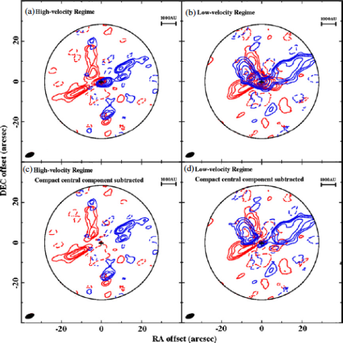
Figure 11: Components of the Outflow. Coordinates are offset from the pointing center. (Figure 7 of Wu et al. 2009)
The second component is an S-shaped structure. It extends along the symmetry axis of the X-shaped component as well as the large scale outflow, but in an opposite orientation. As it literally means, this component is twisted like an ‘S’, although the western arm is not so prominent.
- The compact central component
The third component is a compact, high-velocity outflow very close to the protostars. The authors fitted a 2-d Gaussian structure to this component and made a integrated blue/red-shifted intensity map, which shows a likely outflow feature in the same projected orientation with the X-shaped component and the large scale outflow.
Modeling the outflows
- A Cone-shaped cavity model for the X-shaped component
The authors then move on to construct outflow models for these components. For the X-shaped component, a cone-shaped outflow cavity model is proposed (see Fig. 12 and compare with Fig. 11). By carefully selecting the opening angle of the cone and position angle of the axis, plus assuming a Hubble-like radial expansion, this model can reproduce the X-shaped morphology and the velocity pattern. The origin of this cone is related to a high-velocity and well collimated wind, followed by a low-velocity and wide-angle wind that excavates the cone-shaped cavity. Therefore, what we see as X-shaped structure is actually the inner walls of the cavity. However, this model cannot incorporate the NW arm into the picture.
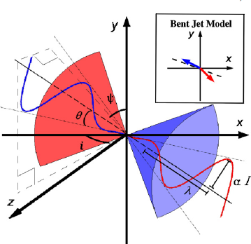
Figure 12: Models from the paper (Figure 10 of Wu et al. 2009)
- Entrained material model of the compact central component
For the compact central component, the authors argue that it is material that has been entrained recently by the jets. After comparing the momentum of this component and that of the optical jets, they found that the jets are able to drive this component. Moreover, the X-ray emission around this component indicates strong shocks, which could be produced by the high-velocity jets as well. Finally, the possibility of infalling motion instead of outflow is excluded, because the velocity gradient is larger than the typical value and rotation should dominate over infall at this scale.
- Three models of the X-shaped component
For the S-shaped component, the authors present the boldest idea in this paper. They present three possible explanations at one go, then analyze their pros and cons in four pages. But before we proceed, do we need to consider other possibilities, such as that this S-shaped component is not interconnected at all, but instead contains two separate outflows from different objects, or that the western arm of the component is not actually part of the outflow but some background or foreground emission? Although the model can reproduce the velocity pattern, it has so many adjustable parameters that we could use it to reproduce anything we like (which reminds me of the story of ‘drawing an elephant with four parameters‘). Anyway, let’s consider the three explanations individually.
- Near and far sides of outflow cavity walls? This possibility is excluded because it cannot be incorporated into the cone-shaped cavity model aforementioned, and cannot explain the S-shaped morphology.
- A precessing outflow? The outflow should be driven by a jet. Then if the jet is precessing, the outflow will also be twisted. The authors considered two scenarios: a straight jet and a bent jet, and found with finely tuned precessing angle and period, the bent jet model can best reproduce the velocity pattern along the symmetry axis. Therefore, the orbital motion between the third protostellar component, which is thought to be the driving source of this jet, and northern protostellar component, is proposed to cause the precession of the jet thus the outflow. A schematic image is shown in Fig 12.
- A winding outflow due to orbital motion? The difference between this explanation and the previous one is that in a precessing outflow the driving source itself is swung by its companion protostar, so the outflow is point symmetric, while in a winding outflow the driving source is unaffected but the outflow is dragged by the gravity of its companion as it proceeds, so it has mirror symmetry with respect to the circumstellar disk plain. Again, if we fine-tune the parameters in this model, we can reproduce the velocity pattern.
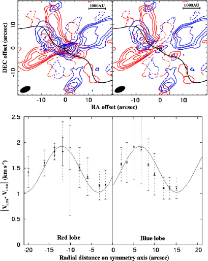
Figure 13: The best-fit model for the S-shaped component, a bent precessing jet. Note the velocity patterns for red/blue lobes are not symmetric (Figure 11 of Wu et al. 2009)
A problem here, however, is although either the precessing jet or the winding outflow model is assumed to be symmetric, the authors use asymmetric velocity patterns to fit the two arms of the S-shaped component (see Fig. 12 and 13 in the paper). In the winding outflow model for instance, in order to best fit the observed velocities, the authors fit the eastern arm starting at a net velocity of 2 km/s at the center, while they fit the western arm starting at ~1.2 km/s. This means the two arms start at different velocities at the center.
Discussion
The nature of X-shaped and S-shaped structures interpreted in this paper is based on the analysis of kinematics and comparison with toy models. However, the robustness of their conclusion suffers from several questions: for example, how to explain the uniqueness of the NW arm in the X-shaped structure? Is the X-shaped structure really a bipolar outflow system, or just two crossing outflows? Why is the compact central component filtered out around the systematic velocity? Is the S-shaped structure really a twisted outflow, or it is two outflow lobes from two separated protostars?
All these questions might be caused by the missing flux problem discussed above. Observations from a single-dish telescope could be combined with the interferometric data to: 1) find the front and back walls of the outflow cavity, given sufficient sensitivity, to confirm that the X-shaped component is interconnected; 2) detect the extended structure around the systematic velocity, thus verify the nature of the compact central component; 3) recover at least part of the flux in the SW arm of the X-shaped component and the west arm of the S-shaped component, and better constrain the models.
Conclusions
Using radio and infrared observations, these three papers together provide a integrated view of jets and outflows around YSOs in L1551. The near infrared observations of Hayashi & Pyo (2009) searched for [Fe II] and H2 features introduced by shocks, and found quite different configurations among the YSOs in this region. Some have complicated IR emission, such as HL/XZ Tau, while others like L1551 NE and IRS5 have well-collimated jets traced by [Fe II]. Among them, L1551 IRS5 is particularly interesting because it shows two parallel jets. The pilot work of Snell et al. (1980) revealed a bipolar molecular outflow traced by 12CO from IRS 5, which is interpreted to be created by a strong stellar wind from the young star. High angular resolution observation by Wu et al. (2009) confirms this outflow component, as well as the presence of another two bipolar outflows originating from the binary, or triple system in IRS 5. All these observations show us that jets and outflows are essential in star formation, no only by transporting the angular momentum so that YSOs can continue accreting, but also by stirring up ambient gas and feeding turbulence into the ISM, which might determine the core mass function as mentioned in Alves et al. 2007.
References
Cudworth, K. M. and Herbig, G. 1979, AJ, 84, 548.
Dopita, M. 1978, ApJ Supp., 37, 117.
Gilmore, W. S. 1978, Ph.D Thesis, University of Maryland
Hayashi, M. and Pyo, T.-S. 2009, ApJ, 694, 582-592.
Hollenback, D. and McKee, C. F. 1989, ApJ, 342, 306-336.
Lim, J. and Takakuwa, S. 2006, ApJ, 653, 1.
Lyons, B. T. 1962, ApJ Supp., 7, 1.
Raymond, J. C. 1979, ApJ Supp., 39, 1.
Reipurth, B., et al. 2000, AJ, 120, 3.
Pineda, J. et al. 2011, ApJ Lett., 739, 1.
Shu, F. H., Adams, F. C., Lizano, S. 1987, ARA&A, 25, 23-81.
Smith, M. D. 1994, A&A, 289, 1.
Snell, R. L. 1979, Ph.D Thesis, University of Texas.
Strom, S. E., Grasdalen, G. L. and Strom, K. M. 1974, ApJ, 191, 111.
Vrba, F. J., Strom, S. E. and Strom, K. M., 1976, AJ, 81, 958.
Wu, P.-F., Takakuwa, S., and Lim, J. 2009, 698, 184-197. Read the rest of this entry »
(where
is the galaxy circular velocity), consistent with simple momentum-conservation expectations. We use our suite of simulations to study the relative contribution of each feedback mechanism to the generation of galactic winds in a range of galaxy models, from Small Magellanic Cloud-like dwarfs and Milky Way (MW) analogues to z ∼ 2 clumpy discs. In massive, gas-rich systems (local starbursts and high-z galaxies), radiation pressure dominates the wind generation. By contrast, for MW-like spirals and dwarf galaxies the gas densities are much lower and sources of shock-heated gas such as supernovae and stellar winds dominate the production of large-scale outflows. In all of our models, however, the winds have a complex multiphase structure that depends on the interaction between multiple feedback mechanisms operating on different spatial scales and time-scales: any single feedback mechanism fails to reproduce the winds observed.We use our simulations to provide fitting functions to the wind mass loading and velocities as a function of galaxy properties, for use in cosmological simulations and semi- analytic models. These differ from typically adopted formulae with an explicit dependence on the gas surface density that can be very important in both low-density dwarf galaxies and high-density gas-rich galaxies.


 rest frequency is roughly 24 GHz, we can find the energy of the transition:
  . This corresponds to an excitation temperature of 1.2 K, which we can also translate into a velocity via
  . A typical molecular cloud temperature is on the order of 20 K, high enough that there should be many molecules in the upper energy state (think of it as a toy-model 2 level system) and hence many upper to lower transitions occurring (leading to emission at 24 GHz).
 . Here, we have a fractional frequency shift
  , and setting
  = 3.9 kHZ/24 GHz leads to the velocity quoted (.049 km/s).
 , where
  is the angular resolution,
  the wavelength of light, and
  the diameter of the aperture (here, the baseline). 24 GHz has
  cm, so with a 1 km baseline the angular resolution is about .05’’ (for comparison, this is 1.3 times the angular resolution of the Hubble Space Telescope at 500 nm).
 describes the shape of the SED)).There will be some intrinsic noise in both amplitude and phase, which you want to eliminate. For a source that has a flat spectrum, you know any bumps you see at a particular frequency are due to noise in the channel at that frequency. This is the purpose of having an amplitude calibrator: typically quasars are used because they have flat spectra.


 and
and  years
years = 20.
= 20. . Here,
  is the
  of the best-fit model for each source. Robitaille et al. acknowledge that this cut-off has no statistical justification: ‘Athough this cut-off is arbitrary, it provides a range of acceptable fits to the eye.’ After taking

 . One has
 ,
, .
.![r \equiv \bigg[ \frac{(n+1)K_n}{4\pi G \lambda ^{1-1/n} } \bigg]^{1/2} \xi](https://s0.wp.com/latex.php?latex=r+%5Cequiv+%5Cbigg%5B+%5Cfrac%7B%28n%2B1%29K_n%7D%7B4%5Cpi+G+%5Clambda+%5E%7B1-1%2Fn%7D+%7D+%5Cbigg%5D%5E%7B1%2F2%7D+%5Cxi&bg=FFFFFF&fg=000000&s=0&c=20201002) ,
, ,
,
![r\equiv \bigg[ \frac{K_I}{4\pi G \lambda} \big]^{1/2}\xi](https://s0.wp.com/latex.php?latex=r%5Cequiv+%5Cbigg%5B+%5Cfrac%7BK_I%7D%7B4%5Cpi+G+%5Clambda%7D+%5Cbig%5D%5E%7B1%2F2%7D%5Cxi&bg=FFFFFF&fg=000000&s=0&c=20201002)
 .
. .
. and
and  , we find
 .
. the equation may be integrated to give
 .
.
 .
.
 eV, called the ‘knee’ and one at
  eV, called the ‘ankle’. Bell’s contribution is the derivation of a cosmic ray power law spectrum via acceleration in the shocks of supernova remnants. Bell’s model did not explain why the ‘ankle’ and the ‘knee’ exist, and to my knowledge the reason for their presence is still an open question. One explanation is that galactic accelerators cannot efficiently produce cosmic rays to arbitrarily high energies. The knee marks the point where galactic accelerators reach their energetic limits. The ankle marks the point where the galactic cosmic ray intensity falls below the intensity of cosmic rays from extragalactic sources, the so called ultra high-energy (UHE) cosmic rays (
 is the energy of the particle as it is injected in the acceleration process and
  is defined to be:
 denotes terms of order
  and higher.
 and
and  are respectively the velocity of the scattering centers. Each are given by:

 is the Alfven speed,
  the mean velocity of scattering centers downstream,
  the shock velocity, and
  the factor by which the gas is compressed at the shock (
 for high Mach number shocks obeying
 is the Alfven Mach number of the shock. In particular, for typical shock conditions this gives us a slope of
  to
to  , in agreement with the observed power law of the cosmic ray spectrum.
 , the background particle distribution, is exactly
  (the Galactic particle distribution) if the shock is moving through undisturbed interstellar gas. This condition is false for objects that generates multiple shock fronts. Also note that due to compression in the shockwave,
  can be many times the galactic value.
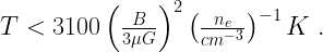

 (better argued in
  and
and  respectively (look at Figure 2 of Bell’s paper, reproduced preceding this paragraph), the energy increase due to one crossing is:
 and
and  are not parallel, the increase per crossing is smaller than that of the parallel shock. However, the particle’s gyration around magnetic field lines would allow the particle to cross the shock multiple times when it drifts close to the shock (remember, the particle’s gyration radius must be large compared to the shock’s width for it to participate in the acceleration process!). In total, Bell claims that these two effects cancel each other out, resulting in the same power law spectrum.
 is the energy in the original region (upstream) and
  is the energy in the downstream region;
  is the velocity at which the particle is crossing from upstream to downstream; and
  is the difference of the velocity between scattering centers upstream and downstream parallel to the shock’s normal (direction of Lorentz boost) given by:
  , where
  is the angle the motion is making with the shock’s normal. Putting this together gives:
 (inverse Lorentz transformation) since we are measuring everything in the frame of the upstream scattering centers. This gives:
 .
. is the momentum of the particle after it crosses and
  is the momentum of the particle before it crosses:


 on the last line. This is the amount of energy the particle possess after it crosses from the upstream to the downstream. The increase in energy is:
 equation that it comes from the difference in velocity of the scattering centers upstream and downstream
  . Therefore, cosmic ray acceleration is literally a process where energetic particles steal energy from the bulk fluid motion!!!
 will have to be changed to
  , giving a minus sign. However, the angle must be inverted,
  , netting another minus sign. The energy change is always positive no matter if the particle crosses from upstream to downstream or downstream to upstream. Particles always gain and never lose energy when the cross a shock!!! In particular, the total energy gain by a particle after many crossings is just the product of a bunch of these
  terms!
 are both measured in the upstream frame. Therefore, the extra minus sign from
 term of the second crossing. It is now obvious to see that this is exactly equation (4) if we Taylor expand the denominator to linear order in
  . Since equation (7) in Bell’s paper only goes to linear order in
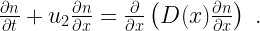
 in the downstream region. The two important mechanisms are advection due to the fluid flow (with advection velocity
  with its flux,
  .
.

 since the advection velocity downstream is
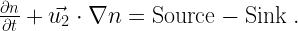
 , we can put diffusion into the Source – Sink term.
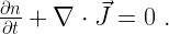
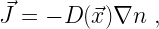
 is called the \textbf{diffusion coefficient} and can vary with respect to position in the shock. Plugging this to the previous equation gives:

 and
and  , since we assume that the advection velocity and diffusion coefficient do not vary perpendicular to the shock’s normal.
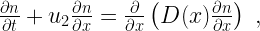


 ? What the heck is the (1,1)
 ). The right panel has zoomed in on the regions with subsonic velocity dispersions, which are bounded in the left panel by the orange contour.
 and hence more coherent velocities; they become less coherent near the YSO, possibly due to feedback.
 ? Why? There’s a very simple

