Author: Yuan-Sen Ting, April 2013
In the remembrance of Boston bombing victims: M. Richard, S. Collier, L. Lu, K. Campell
“Weeds do not easily grow in a field planted with vegetable.
Evil does not easily arise in a heart filled with goodness.”
Dharma Master Cheng Yen.
Related links:
- For more information and interactive demonstrations of the concepts discussed here, see the interactive online software module I developed for the Harvard AY201b course.
Introduction
Although this seminal paper by Gunn & Peterson (1965) comprises only four pages (not to mention, it is in single column and has a large margin!), the authors suggested three ideas that are still being actively researched by astronomers today, namely
- Lyman alpha (Lyα) forest
- Gunn-Peterson trough
- Cosmic Microwave Background (CMB) polarization
Admittedly, they put them in a slightly different context, and the current methods on these topics are much more advanced than what they studied, but one could not ask for more in a four pages note! In the following, we will give a brief overview on these topics, the initial discussion in Gunn & Peterson (1965) and the current thinking/results on these topics. Most of the results are collated from the few review articles/papers in the reference list and we will refer them herein.
Lyman alpha forest
Gunn and Peterson propose using Lyα absorption in the distant quasar spectrum to study the neutral hydrogen in the intergalactic medium (IGM). The quasar acts as the light source, like shining a flashlight across the Universe, and provides a characteristic, relatively smooth spectrum. During the transmission of the light from the quasar to us, intervening neutral hydrogen clouds, along the line of sight to the quasar, cause absorptions on the quasar continuum at the neutral hydrogen HI transition 1215.67Å in the rest frame of the absorbing clouds. Because the characteristic quasar spectrum is well-understood, it’s relatively easy to isolate and study this absorption.
More importantly, in our expanding Universe, the spectrum is continuously redshifted. Therefore the intervening neutral hydrogen at different redshifts will produce absorption at many different wavelengths blueward of the quasars’ Lyα emission. After all these absorptions, the quasar spectrum will have a “forest” of lines (see figure below), hence the name Lyα forest.
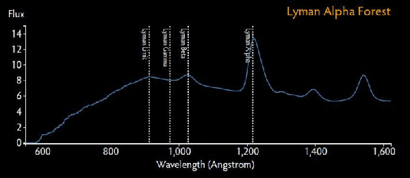
Figure 1. Animation showing a quasar spectrum being continuously redshifted due to cosmic expansion, with various Lyman absorbers acting at different redshifts. From the interactive module.
For a quasar at high redshift, along the line of sight, we are sampling a significant fraction of the Hubble time. Therefore, by studying the Lyα forests, we are essentially reconstructing the history of structure formation. To put our discussion in context, there are two types of Lyα absorbers:
- Low column density absorbers: These absorbers are believed to be the sheetlike-filamentary neutral hydrogen distributed in the web of dark matter formed in the ΛCDM. In this cosmic web, the dark matter filaments are sufficiently shallow to avoid gravitational collapse of the gas but deep enough to prevent these clouds of the inter- and proto-galactic medium from dispersing.
- High column density absorbers: these are mainly due to intervening galaxies/proto-galaxies such as the damped Lyα systems. As opposed to the low column density absorbers, since galaxies are generally more metal rich than the filamentary gas; the absorption of Lyα due to these systems will usually be accompanied by some characteristic metal absorption lines. There will also be an obvious damping wing visible in the Voigt profile of the Lyα line, hence the name damped Lyα system.
Since our discussion here focuses on the IGM, although the high column density absorbers are extremely important to detect high redshift galaxies, for the rest of the discussion in this post, we will only discuss the former.
Low column density absorbers
So, what can we learn about neutral hydrogen in the Universe by looking at Lyα forests? With a large sample of high redshift quasar spectra, we can bin up the absorption lines due to intervening clouds of the same redshift. This allows us to study the properties of gas at that distance (at that time in the Universe’s history), and learn about the evolution of the IGM. In this section, we summarize some of the crucial properties that are relevant in our later discussion:
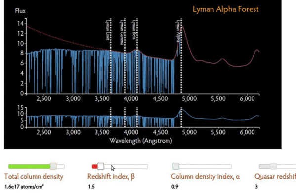
Figure 2. Animation illustrating the effect of the redshift index on the quasar absorption spectrum. A higher index means more closely spaced absorption near the emission peak. From the interactive module.
It turns out that the properties of the IGM can be rather well described by power laws. If we define n(z) as the number density of clouds as a function of redshift z, and N(ρ) as the number density of clouds as a function of column density ρ. It has been observed that [see Rauch (1998) for details],

Note that, in order to study these distributions, ideally, high resolution spectroscopy is needed (FWHM < 25 kms-1) such that each line is resolved.
There is an upturn in the redshift power law index at high redshift. This turns out to be relevant in the discussion of the Gunn-Peterson trough. We will discuss this later. It has also been shown, via cosmological hydrodynamic simulations, that the ΛCDM model is able to reproduce to the observed power laws.
But we can learn about more than just gas density. The Doppler widths of Lyα line are consistent with the photoionization temperature (about 104 K). This suggests that the neutral hydrogen gas in the Lyα clouds is in photoionization equilibrium. In other words, the photoionization (i.e. heating) due to the UV background photons is balanced by cooling processes via thermal bremsstrahlung, Compton cooling and the usual recombination. Photoionization equilibrium allows us to calculate how many photons have to be produced, either from galaxies or quasars, in order to maintain the gas at the observed temperature. Based on this number of photons, we can deduce how many stars were formed at each epoch in the history of the Universe.
We’ve been relying on the assumption that these absorbers are intergalactic gas clouds. How can we be sure they’re not actually just outflows of gas from galaxies? This question has been tackled by studying the two point correlation function of the absorption lines. In a nutshell, two point correlation function measures the clustering of the absorbers. Since galaxies are highly clustered, at least at low redshift, if the low density absorbers are related to the outflow of galaxies, one should expect clustering of these absorption signals. The studies of Lyα forest suggest that the low column density absorbers are not clustered as strongly as galaxies, favoring the interpretation that they are filamentary structures or intergalactic gas [see Rauch (1998) for details].
However this discussion is only valid in the relatively recent Universe. When we look further, and therefore study the earliest times, there are less photons and correspondingly more neutral hydrogen atoms. With more and more absorption, eventually the lines in the forest become so compact and deep that the “forest” becomes a “trough”.
Gunn-Peterson trough
In their original paper in 1965, Gunn and Peterson estimated how much absorption there should be in a quasar spectrum due to the amount of hydrogen in the Universe. The amount of absorption can be quantified by optical depth which is a measure of transparency. A higher optical depth indicates more absorption due to the neutral hydrogen. Their cosmological model during that time is obsolete now, but their reasoning and derivation are still valid, one can still show that the optical depth
With a modern twist on the cosmological model, the optical depth of neutral hydrogen at each redshift can be estimated to be
where z is the redshift, λ is the transition wavelength, e is the electric charge, me is the electron mass, f is the oscillatory strength of the electronic state transition from N=1 to 2, H(z) is the Hubble constant, h is the dimensionless Hubble’s parameter, Ωb is the baryon density of the Universe, Ωm is the dark matter density, nHI is the number density of neutral hydrogen and nH is the total number density of both the neutral and ionized hydrogen.
Since optical depth is proportional to the density of neutral hydrogen, and the transmitted flux ratio decreases exponentially with respect to the optical depth, even a tiny neutral density fraction, nHI/nH=10-4 (i.e. one neutral hydrogen atom in ten thousands hydrogen atoms) will give rise to complete Lyα absorption. In other words, the transmitted flux should be zero. This complete absorption is known as the Gunn-Peterson trough.
In 1965, Gunn and Peterson performed their calculation assuming that most hydrogen atoms in the Universe are neutral. From their calculation, they expected to see a trough in the quasar (redshift z∼3) data they were studying. This was not the case.
In order to explain the observation, they found that the neutral hydrogen density has to be five orders of magnitude smaller than expected. They came to the striking conclusion that most of the hydrogen in the IGM exists in another form — ionized hydrogen. Lyman series absorptions occur when a ground state electron in a hydrogen atom jumps to a higher state. Ionized hydrogen has no electrons, so it does not absorb photons at Lyman wavelengths.
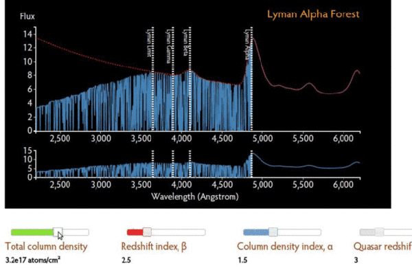
Figure 3. Animation illustrating Gunn-Peterson trough formation. The continuum blueward of Lyα is drastically absorbed as the neutral hydrogen density increases. From the interactive module.
Gunn and Peterson also showed that since the IGM density is low, radiative ionization (instead of collisional) is the dominant source to maintain such a level of ionization. What an insight!
The history of reionization
In modern astronomy language, we refer to Gunn and Peterson’s observation by saying the Universe was “reionized”. Combined with our other knowledge of the Universe, we now know the baryonic medium in the Universe went through three phases.
- In the beginning of the Universe (z>1100), all matter is hot, ionized, optically thick to Thomson scattering and strongly coupled to photons. In other words, the photons are being scattered all the time. The Universe is opaque.
- As the Universe expands and cools adiabatically, the baryonic medium eventually recombines, in other words, electrons become bound to protons and the Universe becomes neutral. With matter and radiation decoupled, the CMB radiation is free to propagate.
- At some point, the Universe gets reionized again and most neutral hydrogen becomes ionized. It is believed that the first phase of reionization is confined to the Stromgren spheres of the photoionization sources. Eventually, these spheres grow and overlap, completing the reionization. Sources of photoionizing photons slowly etch away at the remaining dense, neutral, filamentary hydrogen.
When and how reionization happened in detail are still active research areas that we know very little about. Nevertheless, studying the Gunn-Peterson trough can tell us when reionization completed. The idea is simple. As we look at quasars further and further away, there should be a redshift where the quasar sources were emitting before reionization completed. These quasar spectra should show Gunn-Peterson troughs.
Pinning down the end of reionization
The first confirmed Gunn-Peterson trough was discovered by Becker et al. (2001). As shown in the figure below, the average transmitted flux in some parts of the quasar spectrum is zero.
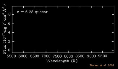

Figure 4. The first confirmed detection of the Gunn-Peterson trough (top panel, where the continuum goes to zero flux due to intervening absorbers), from a quasar beyond z = 6. The bottom panel shows that the quasar after z = 6 has non-zero flux at all parts. Adapted from Becker et al. (2001).
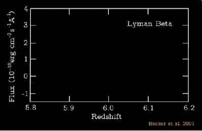
Figure 5. The close up spectra of the redshift z>6 quasar. In the regions corresponding to the absorbers redshift 5.95 <z< 6.16 (i.e. the middle regions), the transmitted flux is consistent with zero flux. This indicates a strong increment of neutral fraction at z>6. Note that, near the quasar (the upper end), there is transmitted flux. This is mostly owing to the fact that the neutral gas near the quasar is ionized by the quasar emission and therefore the Gunn-Peterson trough is suppressed. This is also known as the proximity effect. As we go to the regions corresponding to lower redshift, there is also apparent transmitted flux, indicating the neutral fraction decreases significantly.
Could this be due to the dense interstellar medium of a galaxy along the line of sight, rather than IGM absorbers? A few lines of evidence refute that idea. First, metal lines typically seen in galaxies (even in the early Universe) are not observed at the same redshift as the Lyman absorptions. Second, astronomers have corroborated this finding using several other quasars. We see these troughs not just a few particular wavelengths in some of the quasar spectra (as you might expect for scattered galaxies), but rather the average optical depth steadily grows, versus a simple extrapolation of how it grows at low redshifts, starting at redshift of z∼6 (see figure below). The rising optical depth is due to the neutral hydrogen fraction rising dramatically beyond z>6.
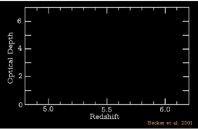
Figure 6. Quasar optical depth as a function of redshift. The observed optical depth exceeds the predicted trend (solid line), suggesting reionization. Adapted from Becker et al. (2001).
Similar studies using high redshift z>5 quasars confirm a dramatic increases in the IGM neutral fraction from nHI/nH=10-4 at z<6, to nHI/nH>10-3–0.1 at z∼6. At z>6, complete absorption troughs begin to appear.

Figure 7. A more recent compilation of Figure 6 from Fan et al. (2006). Note that the sample variance increases rapidly with redshift. This could be explained by the fact that high redshift star-forming galaxies, which likely provide most of the UV photons for reionization, are highly clustered, therefore reionization is clumpy in nature.
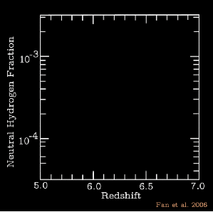
Figure 8. A similar plot, but translating the optical depth into volume-averaged neutral hydrogen fraction of the IGM. The solid points and error bars are measurements based on 19 high redshift quasars. The solid line is inferred from the reionization simulation from Gnedin (2004) which includes the overlapping stage to post-overlapping stage of the reionization spheres.
But it’s important to note that, because even a very small amount of neutral hydrogen in the IGM can produce optical depth τ≫1 and cause the Gunn-Peterson trough, this observational feature saturates very quickly and becomes insensitive to higher densities. That means that the existence of a Gunn-Peterson trough by itself does not prove that the object is observed prior to the start of reionization. Instead, this technique mostly probes the later stages of cosmic reionization. So the question now is: when does reionization get started?
The start of reionization
Gunn and Peterson told us not only how to probe the end of reionization through the Gunn-Peterson trough, but also how to probe the early stages of reionization using the polarization of the CMB. They discussed the following scenario: if the Universe starts to be reionized at certain redshift, then beyond this, the background distant light sources should experience Thomson scattering.
Thomson scattering is the scattering between free electrons and photons. Recall the fact that due to Thomson scattering by the surrounding nebulae, the starlight undergoes this scattering will be polarized (due to the angle dependence of Thomson scattering). By the same analogy, the CMB, after Thomson scattering off the ionized IGM, is polarized.
As opposed to the case of the Gunn-Peterson troughs, the Thomson scattering results from light interacting with the ionized fraction of hydrogen, not the neutral fraction. Therefore, the large scale polarization of the CMB can be regarded as a complimentary probe of reionization. The CMB polarization detection by Wilkinson Microwave Anisotropy Probe (WMAP) space telescope suggests a significant ionization fraction extending to much earlier in the cosmic history, with z∼11±3 (see figure below). This implies that reionization is a process which starts at some point between z∼8–14 and ends at z∼6–8. This means that cosmic reionization appears to be quite extended in time. This is in contrast to recombination, when electrons became bound to protons, which occurred over a very narrow range in time (z=1089±1).
In summary, a very crude chart on reionization using Gunn-Peterson trough and CMB polarization is shown below.
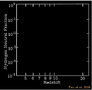
Figure 9. The volume-averaged neutral fraction of the IGM versus redshift measured using various techniques, including CMB polarization and Gunn-Peterson troughs.
So far, we have left out the discussion of Lyβ, Lyγ absorptions as well as the cosmic Stromgren sphere technique as shown in the figure above. We will now fill in the details before proceeding to the suspects of reionization.
How about Lyman beta and Lyman gamma
When people talk about the Lyα forest, sometimes it could be an over-simplification. Besides Lyα, other neutral hydrogen transitions such as Lyβ and Lyγ, play a crucial role. Sometimes we can even study the neutral helium Lyα (note that Lyα only designates the transition from electronic state N=1 to 2). We now first look at the advantages and also impediments to include Lyβ and Lyγ absorption lines in the study of the IGM.
- Recall the formula for the optical depth: τ∝f λ. Due to the decrease in oscillator strength and also the wavelength, for the same neutral fraction density, the Gunn-Peterson optical depths of Lyβ and Lyγ are 6.2 and 17.9 times smaller than Lyα. Having smaller optical depth means that the absorption lines will only saturate at higher neutral fraction/density. Note that once a line is saturated, a large change in column density will only induce a small change in apparent line width. In other words, we are in the flat part of the curve of growth. In this case, the column densities are relatively difficult to measure. Since Lyβ and Lyγ have a smaller optical depths, they could provide more stringent constraints on the IGM ionization state and density when Lyα is saturated. Especially in the case of Gunn-Peterson trough, as we have shown in the figures above, the ability to detect Lyβ and Lyγ is crucial to study reionization.
- Note that, given the same IGM clouds, the absorption of Lyα will also be accompanied by Lyβ and Lyγ absorptions. Since Lyα has a stronger optical depth, it has broader wings in the Voigt profile and has a higher chance to blend with the other lines. Therefore, simultaneous fits to higher order Lyman lines could help to deblend these lines.
- As the redshift of quasar increases, there is a substantial overlapping region between Lyβ with Lyα, and so forth. Disentangling which absorption line is due to Lyα and which is due to higher order absorptions is difficult within these regions. Due to this limitation, the study of Lyγ, and higher order lines, is rare.
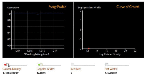
Figure 10. The left-hand panel shows the Voigt profile of Lyα absorption line. The animation shows that when the line is saturated, a large change in column density will only induce a small change in the equivalent width (right-hand panel). This degeneracy makes the measurement of column density very difficult when the absorption line is saturated. From the interactive module.
Figure 11. Animation showing the Lyα forest including Lyα and Lyβ absorption lines. One can see that there is a substantial overlapping of Lyα absorption lines onto the the Lyβ region. Therefore, the study of higher order absorptions is very difficult in practice. From the interactive module.
Probing even higher neutral fraction
In some of the plots above, we have seen that as the neutral fraction increases, Lyα starts to saturate and can only give a moderate lower bound on the optical depth and the neutral fraction. For higher neutral fraction, we have to use Lyβ and Lyγ. It is also clear that even Lyγ will get saturated very quickly. Are there other higher density probes?
Yes, there are other probes! At high neutral fraction, the quasar in this kind of environment resembles a scaled-up version of a O/B type star in a dense neutral hydrogen region (although the latter medium is mostly in molecules, and the former is in atoms). Luminous quasars will produce a highly ionized HII region and create the so called cosmic Stromgren spheres. These cosmic Stromgren spheres could have physical size of about 5 Mpc owing to the extreme luminosity of the quasars.
Measurements of cosmic Stromgren spheres are sensitive to a much larger neutral fraction than the one that Lyγ can probe. However, on the flip side of the coin, they are subjected to many systematics that one could easily imagine, including the three-dimension geometry of the quasar emission, age of the quasar, the clumping factor of the surrounding materials, etc. This explains the large error bar in the reionization chart above.
How about helium absorption
Although hydrogen is the most abundant element in the Universe, we also know that helium constitutes a large fraction of the Universe. A natural question to ask: how about helium?
As neutral helium has a similar ionization potential and recombination rate compared to neutral hydrogen, it is believed that neutral helium reionization is likely to happen at a similar time together with neutral hydrogen. On the other hand, the ionized HeII has a higher ionization potential, and its reionization is observed to happen at lower redshift, about z∼3. The fact that ionized helium has a higher ionization potential is crucial in disentangling the UV background sources. We will discuss this in detail when we talk about the suspects. In this section, we will discuss some potentials and impediments of the usage of helium Lyα.
- Helium and hydrogen have different atomic masses. Note that the bulk motion and thermal motion in gas both contribute to the line broadening. However bulk motions are insensitive to the atomic masses whereas the thermal motion velocities go as 1/√μ, where μ is the mean atomic mass. By comparing the broadening of the HeII 304Å and HI 1215Å lines, it is in principle possible to use the difference in atomic masses to measure the contribution from the bulk and thermal motions to the line broadening, separately. Therefore, the theories of the IGM kinematics can be, in principle, be tested. The usefulness of this approach however is remained to be seen.
- Since ionized helium has a higher ionization potential (Lyman Limit at 228Å) than the neutral hydrogen (Lyman Limit at 912Å), the relative ionization fraction is a sensitive probe of the spectral shape of the UV background. For instance, the contribution from quasars will provide harder spectra than the soft stellar sources and is able to doubly ionize helium.
- Although helium Lyα forest is awesome, only a small fraction of all quasars are suitable for the search of HeII absorption. The short wavelength of 304Å of Lyman alpha line for ionized helium requires the quasar to be redshifted significantly in order to enter the optical band such that we have enough high resolution spectroscopic instrument to detect it. Furthermore, it is important to note that the helium Lyα line has smaller wavelength than the neutral hydrogen Lyman Limit. As shown in the interactive module, the bound-free absorption beyond the Lyman Limit, as especially at the presence of high column density absorber, will create a large blanketing of lines. This renders the large majority of quasars useless for a HeII search even they might be redshifted enough into the optical band.
The suspects — who ionized the gas?
We have discussed enough on the technologies to catch the suspects. So we will now go back to the main question on reionization. Who did it? As we have discussed earlier in this post, the IGM is believed to have been reionized early in the Universe’s history via photoionization. Who produced all the high energy, ionizing photons? There are two natural suspects:
- Star-forming galaxies
- Quasars
It has been argued that soft sources like star-forming galaxies have to be the dominant sources owing to the fact that there are not many quasars in the early Universe. The Sloan Digital Sky Survey (SDSS) has shown a steep decline in the number of quasars after its peak at z=2.5. If most quasars formed after this epoch, could they play a significant role in the reionization of the Universe, which seems to have completed as early as z∼6.
Taking a closer look at this problem, Faucher-Giguère et al. (2008) made an independent estimate of the photoionization contribution from quasars. In their study, they consider Lyα forests optical depth at redshift 2<z<4.2 from 86 high resolution quasar spectra.
The idea to estimate the fractional contribution from quasars has been described earlier in this post, we will iterate with more details here. Only quasars can produce the very high energy (∼50 eV) photons necessary to doubly ionize helium. Therefore, the luminosity of sources at ∼50 eV can directly tell us the contribution from quasars. By assuming a spectral index for the spectral energy distribution, one can then extrapolate to the lower energies and infer the photoionization rate at the energy range that is relevant to the HI ionization. They show that at most only about 20 per cent of these photons could come from quasars.
Beside showing quasars cannot be the main suspect, Faucher-Giguère et al. also use the Lyα forests to derive the star formation rate indirectly. We have discussed that the absorbers are in photoionzation equilibrium. With this assumption, the authors use the Lyα opacity depth to derive the photoionization rate at different redshifts. With the photoionization rate, they turn that into UV emissivity from the star-forming galaxies and then infer the star formation rate in galaxies at different times in the history of the Universe.
The figure below shows that the derived hydrogen photoionization rate is remarkably flat over the history of the Universe. This suggests that there should be a roughly constant photoionizing source over a large range of cosmic history. This is only possible if the star formation rate in galaxies continues to be high in the early Universe, at high redshift (z∼2.5–4) since the contribution from quasars only begins at this redshift. As the figure shows, such a star formation rate is consistent with the simulation of Hernquist & Springel (2003).
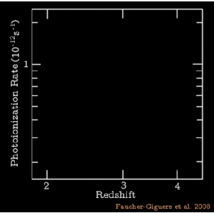
Figure 12. Observations of the hydrogen photoionization rate compared to the best-fitting model from Hernquist & Springel (2003). This suggests that the combination of quasars and stars alone may account for the photoionization. Adapted from Faucher-Giguère et al. (2008).
But there is another way to trace the history of star formation — by directly counting up the number and size of galaxies at different redshifts, using photometric surveys. It turns out that the results from these direct surveys, as performed by Hopkins & Beacom (2006) for example, are in tension with indirect approach. The photometric surveys suggest that the star formation rate decreases after z>2.5 [Prof Hans-Walter Rix once wittily quoted this as the Universe gets tenured at redshift z∼2.5], like in the figure below. The results says that both the major photoionization machines (quasars and stars in galaxies) would be in decline after z>2.5.

Figure 13. Like Figure 12 above, but now using the models of Hopkins & Beacom (2006) where the star formation history is inferred from photometric surveys.
If the photometric surveys are right, Faucher-Giguère et al. strongly suggest that the Universe could not provide enough photons to reionize the intergalactic medium. So, why are there two different observational results?
To sum up this section, by studying Lyα forests, Faucher-Giguère et al. argue that
- Star-forming galaxies are the major sources of photoionization, although quasars can contribute as much as 20 per cent.
- The star formation rate has to be higher than the one estimated observationally from the photometric surveys to provide the required photons.
How the suspect did it
Although the Faucher-Giguère et al. results suggest that star-forming galaxies are the major sources of photoionization, exactly how these suspects actually did it is not clear. The discrepancy between direct and indirect tracers of the star formation history of the Universe might be reconcilable. Observations of star-forming galaxies are plagued with uncertainties, many of which are still areas of active research. Among the major uncertainties are:
- The star formation rate of galaxies at high redshift. We cannot observe galaxies that are faint and far away. How many photons could they provide? Submillimetre observations in near future could shed more light on this due to their amazing negative K-correction and the ability to observe gas and dust in high redshift galaxies.
- Starburst galaxies create dust, and dust can obscure observation. Infrared and submillimetre observations are crucial to detect these faint galaxies. It is believed that perhaps most of the ionizing photons come from these unassuming, hard-to-detect galaxies, because they are likely individually small and dim but collectively numerous.
- IGM clumping factor. In other words, how concentrated is the material surrounding the galaxies? This factor could affect the fraction of ionizing photons escaping into the IGM.
In short, it is possible that the star formation did indeed begin way back in the cosmic history, at z>2.5, but we underestimated it in the photometric surveys due to these uncertainties. In this case, all the results from simulations, Lyα forests, and photometric surveys could fit together.
Any other suspects on loose
We have now two suspects in custody. The remaining question: are there any suspects on loose? To answer this question, some other interesting proposals were raised, among them:
- High-energy X-ray photons from supernova remnants or microquasars at high redshift. This is possible, but its contribution might overestimate the soft X-ray background that we observe today.
- Neutrino is believed to gain their mass through the seesaw mechanism. One of the potential ingredient of this mechanism is the sterile neutrino. Reionization by decaying sterile neutrinos cannot be completely ruled out yet. That said, since there is no confirmed detection of sterile neutrino in particle physics experiments, one should not take this possibility too seriously and blow one own mind.
In summary, we cannot be 100 per cent sure, but other suspect other that quasars and stellar sources is unlikely.
So what have we learned?
To summarize what we have discussed in this post:
- Non-detection can be a good thing. The non-detection of the Gunn-Peterson trough in the early days demonstrated that the IGM is mostly in an ionized state.
- The Lyα forest gives us a 3D picture of the IGM.
- The Gunn-Peterson trough provides a direct probe on the end stage of the reionization.
- CMB radiation polarization suggests when the process of reionization began, and shows that reionization is a process extended in time.
- Star-forming galaxies are likely to be responsible for the reionization, but how they exactly did it is a question still under investigation.
References
- Becker R. H. et al., 2001, AJ, 122, 2850
- Fan X., Carilli C. L., Keating B., 2006, ARA&A, 44, 415
- Faucher-Giguère C.-A., Lidz A., Hernquist L., Zaldarriaga M., 2008, ApJ, 688, 85
- Faucher-Giguère C.-A., Prochaska J. X., Lidz A., Hernquist L., Zaldarriaga M., 2008, ApJ, 681, 831
- Gunn J. E., Peterson B. A., 1965, ApJ, 142, 1633
- Hernquist L, Springel V., 2003, MNRAS, 341, 1253
- Hopkins A. M., Beacom J. F., 2006, ApJ, 651, 142
- Rauch M., 1998, ARA&A, 36, 267
