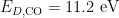
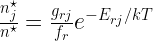
Stromgren Sphere: An example “chalkboard derivation”
(updated for 2013)
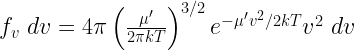
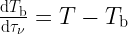
The Stromgren sphere is a simplified analysis of the size of HII regions. Massive O and B stars emit many high-energy photons, which will ionize their surroundings and create HII regions. We assume that such a star is embedded in a uniform medium of neutral hydrogen. A sphere of radius r around this star will become ionized; r is called the “Stromgren radius”. The volume of the ionized region will be such that the rate at which ionized hydrogen recombines equals the rate at which the star emits ionizing photons (i.e. all of the ionizing photons are “used up” re-ionizing hydrogen as it recombines)
The recombination rate density is  , where
  is the recombination coefficient (in
  and
and  is the number density (assuming fully ionized gas and only hydrogen, the electron and proton densities are equal). The total rate of ionizing photons (in photons per second) in the volume of the sphere is
  . Setting the rates of ionization and recombination equal to one another, we get
 , and solving for r,

Typical values for the above variables are  ,
,  and
and  , implying Stromgren radii of 10 to 100 pc. See the journal club (2013) article for discussion of Stromgren’s seminal 1939 paper.
How do we know there is an ISM?
(updated for 2013)
Early astronomers pointed to 3 lines of evidence for the ISM:
- Extinction. The ISM obscures the light from background stars. In 1919, Barnard (JC 2011, 2013) called attention to these “dark markings” on the sky, and put forward the (correct) hypothesis that these were the silhouettes of dark clouds. A good rule of thumb for the amount of extinction present is 1 magnitude of extinction per kpc (for typical, mostly unobscured lines-of-sight).
- Reddening. Even when the ISM doesn’t completely block background starlight, it scatters it. Shorter-wavelength light is preferentially scattered, so stars behind obscuring material appear redder than normal. If a star’s true color is known, its observed color can be used to infer the column density of the ISM between us and the star. Robert Trumpler first used measurements of the apparent “cuspiness” and the brighnesses of star clusters in 1930 to argue for the presence of this effect. Reddening of stars of “known” color is the basis of NICER and related techniques used to map extinction today.
- Stationary Lines. Spectral observations of binary stars show doppler-shifted lines corresponding to the radial velocity of each star. In addition, some of these spectra exhibit stationary (i.e. not doppler-shifted) absorption lines due to stationary material between us and the binary system. Johannes Hartmann first noticed this in 1904 when investigating the spectrum of
 Orionis: “The calcium line at
  [angstroms] exhibits a very peculiar behavior. It is distinguished from all the other lines in this spectrum, first by the fact that it always appears extraordinarily week, but almost perfictly sharp… Closer study on this point now led me to the quite surprising result that the calcium line… does not share in the periodic displacements of the lines caused by the orbital motion of the star”
Helpful References: Good discussion of the history of extinction and reddening, from Michael Richmond.
A Sense of Scale
(updated for 2013)
How dense (or not) is the ISM?
- Dense cores:
- Typical ISM:
- This room: 1 mol / 22.4L

- XVH (eXtremely High Vacuum) — best human-made vacuum:

- Density of stars in the Milky Way:

In other words, most of the ISM is at a density far below the densities and pressures we can reproduce in the lab. Thus, the details of most of the microphysics in the ISM are still poorly understood. We also see that the density of stars in the Galaxy is quite small – only a few times the average particle density of the ISM.
See also the interstellar cloud properties table and conversions between angular and linear scale.
Density of the Milky Way’s ISM
(updated for 2013)
How do we know that  in the ISM? From the rotation curve of the Milky Way (and some assumptions about the mass ratio of gas to gas+stars+dark matter), we can infer
Maps of HI and CO reveal the extent of our galaxy to be
 kpc
kpc
 pc (scale height of HI)
This applies an approximate volume of

Which, yields a density of

Density of the Intergalactic Medium
(updated for 2013)
From cosmology observations, we know the universe to be very nearly flat ( ). This implies that the mean density of the universe is
  .
.
This places an upper limit on the density of the Intergalactic Medium.
Composition of the ISM
(updated for 2013)
- Gas: by mass, gas is 60% Hydrogen, 30% Helium. By number, gas is 88% H, 10% He, and 2% heavier elements
- Dust: The term “dust” applies roughly to any molecule too big to name. The size distribution is biased towards small (0.2
 m) particles, with an approximate distribution
  . The density of dust in the galaxy is
- Cosmic Rays: Charged, high-energy (anti)protons, nuclei, electrons, and positrons. Cosmic rays have an energy density of
 . The equivalent mass density (using E = mc^2) is
- Magnetic Fields: Typical field strengths in the MW are
 . This is strong enough to confine cosmic rays.
Bruce Draine’s List of constituents in the ISM:
(updated for 2013)
- Gas
- Dust
- Cosmic Rays*
- Photons**
- B-Field
- Gravitational Field
- Dark Matter
*cosmic rays are highly relativistic, super-energetic ions and electrons
**photons include:
- The Cosmic Microwave Background (2.7 K)
- starlight from stellar photospheres (UV, optical, NIR,…)
 from transitions in atoms, ions, and molecules
- “thermal emission” from dust (heated by starlight, AGN)
- free-free emission (bremsstrahlung) in plasma
- synchrotron radiation from relativistic electrons
 -rays from nuclear transitions
His list of “phases” from Table 1.3:
- Coronal gas (Hot Ionized Medium, or “HIM”):
 . Shock-heated from supernovae. Fills half the volume of the galaxy, and cools in about 1 Myr.
- HII gas: Ionized mostly by O and early B stars. Called an “HII region” when confined by a molecular cloud, otherwise called “diffuse HII”.
- Warm HI (Warm Neutral Medium, or “WNM”): atomic,
 .
.  . Heated by starlight, photoelectric effect, and cosmic rays. Fills ~40% of the volume.
- Cool HI (Cold Neutral Medium, or “CNM”).
 . Fills ~1% of the volume.
- Diffuse molecular gas. Where HI self-shields from UV radiation to allow
 formation on the surfaces of dust grains in cloud interiors. This occurs at
  .
.
- Dense Molecular gas. “Bound” according to Draine (though maybe not).
 . Sites of star formation. See also Bok Globules (JC 2013).
- Stellar Outflows.
 . Winds from cool stars.
These phases are fluid and dynamic, and change on a variety of time and spatial scales. Examples include growth of an HII region, evaporation of molecular clouds, the interface between the ISM and IGM, cooling of supernova remnants, mixing, recombination, etc.
Topology of the ISM
(updated for 2013)
A grab-bag of properties of the Milky Way
- HII scale height: 1 kpc
- CO scale height: 50-75 pc
- HI scale height: 130-400 pc
- Stellar scale height: 100 pc in spiral arm, 500 pc in disk
- Stellar mass:

- Dark matter mass:
- HI mass:

- H2 mass (inferred from CO):

- HII mass:
- -> total gas mass
 (including He).
- Total MW mass within 15 kpc:
 (using the Galaxy’s rotation curve). About 50% dark matter.
So the ISM is a relatively small constituent of the Galaxy (by mass).
The Sound Speed
(updated for 2013)
The speed of sound is the speed at which pressure disturbances travel in a medium. It is defined as
 ,
,
where  and
and  are pressure and mass density, respectively. For a polytropic gas, i.e. one defined by the equation of state
  , this becomes
  . is the adiabatic index (ratio of specific heats), and
  describes a monatomic gas.
For an isothermal gas where the ideal gas equation of state  holds,
  . Here,
  is the mean molecular weight (a factor that accounts for the chemical composition of the gas), and
  is the hydrogen atomic mass. Note that for pure molecular hydrogen
  . For molecular gas with ~10% He by mass and trace metals,
  is often used.
A gas can be approximated to be isothermal if the sound wave period is much higher than the (radiative) cooling time of the gas, as any increase in temperature due to compression by the wave will be immediately followed by radiative cooling to the original equilibrium temperature well before the next compression occurs. Many astrophysical situations in the ISM are close to being isothermal, thus the isothermal sound speed is often used. For example, in conditions where temperature and density are independent such as H II regions (where the gas temperature is set by the ionizing star’s spectrum), the gas is very close to isothermal.
Hydrogen “Slang”
(updated for 2013)
Lyman limit: the minimum energy needed to remove an electron from a Hydrogen atom. A “Lyman limit photon” is a photon with at least this energy.
 ,
,
where  is the Rydberg constant, which has units of
  . This energy corresponds to the Lyman limit wavelength as follows:
 .
.
Lyman series: transitions to and from the n=1 energy level of the Bohr atom. The first line in this series was discovered in 1906 using UV studies of electrically excited hydrogen gas.
Balmer series: transitions to and from the n=2 energy level. Discovered in 1885; since these are optical transitions, they were more easily observed than the UV Lyman series transitions.
There are also other named series corresponding to higher n. Examples include Paschen (n=3), Brackett (n=4), and Pfund (n=5). The lowest energy (longest wavelength) transition of a series is designated , the next lowest energy is  , and so on. For example, the transition from n=2 to 1 is Lyman alpha, or
  , while the transition from n=7 to 4 is Brackett gamma, or
  . The wavelength of a given transition can be computed via the Rydberg equation:
 ,
,
where  and
and  are the initial and final energy levels of the electron, respectively. See this handout for a pictorial representation of the low n transitions in hydrogen. Note that the Lyman (or Balmer, Paschen, etc.) limit can be computed by inserting
  in the above equation.
The Lyman continuum corresponds to the region of the spectrum near the Lyman limit, where the spacing between energy levels becomes comparable to spectral line widths and so individual lines are no longer distinguishable. Such continua exist for each series of lines.
Chemistry
(updated for 2013)
See Draine Table 1.4 for elemental abundances for the Sun (and thus presumably for the ISM near the Sun).
By number:  ;
;
by mass:  .
.
However, these ratios vary by position in the galaxy, especially for heavier elements (which depend on stellar processing). For example, the abundance of heavy elements (Z ≥ 6, i.e. carbon and heavier) is twice as low at the sun’s position than in the Galactic center. Even though metals account for only 1% of the mass, they dominate most of the important chemistry, ionization, and heating/cooling processes. They are essential for star formation, as they allow molecular clouds to cool and collapse.
Dissociating molecules takes less energy than ionizing atoms, in general. For example:
 (UV transition)
 ,
,
where  and
and  are the ionization and dissociation energies, respectively. We can see that it is much easier to dissociate molecular hydrogen than to ionize atomic hydrogen; in other words, atomic H will survive a harsher radiation field than molecular H. The above numbers thus set the structure of molecular clouds in the interstellar radiation field; a large amount of molecular gas needs to gather together in order to allow it to survive via the process of self-shielding, in which a thick enough column of gas exists such that at some distance below the surface of the cloud all of the energetic photons have already been absorbed. Note that the high dissociation energy of CO is a result of the triple bond between the carbon and oxygen atoms. CO is a very important coolant in molecular clouds.
Measuring States in the ISM
(updated for 2013)
There are two primary observational diagnostics of the thermal, chemical, and ionization states in the ISM:
- Spectral Energy Distribution (SED; broadband low-resolution)
- Spectrum (narrowband, high-resolution)
SEDs
Very generally, if a source’s SED is blackbody-like, one can fit a Planck function to the SED and derive the temperature and column density (if one can assume LTE). If an SED is not blackbody-like, the emission is the sum of various processes, including:
- thermal emission (e.g. dust, CMB)
- synchrotron emission (power law spectrum)
- free-free emission (thermal for a thermal electron distribution)
Spectra
Quantum mechanics combined with chemistry can predict line strengths. Ratios of lines can be used to model “excitation”, i.e. what physical conditions (density, temperature, radiation field, ionization fraction, etc.) lead to the observed distribution of line strengths. Excitation is controlled by
- collisions between particles (LTE often assumed, but not always true)
- photons from the interstellar radiation field, nearby stars, shocks, CMB, chemistry, cosmic rays
- recombination/ionization/dissociation
Which of these processes matter where? In class (2011), we drew the following schematic.

A schematic of several structures in the ISM
Key
A: Dense molecular cloud with stars forming within
 (measured, e.g., from line ratios)
- gas is mostly molecular (low T, high n, self-shielding from UV photons, few shocks)
- not much photoionization due to high extinction (but could be complicated ionization structure due to patchy extinction)
- cosmic rays can penetrate, leading to fractional ionization:
 , where is the ion density (see Draine 16.5 for details). Measured values for
  (the electron-to-neutral ratio, which is presumed equal to the ionization fraction) are about
  .
.
- possible shocks due to impinging HII region – could raise T, n, ionization, and change chemistry globally
- shocks due to embedded young stars w/ outflows and winds -> local changes in T, n, ionization, chemistry
- time evolution? feedback from stars formed within?
B: Cluster of OB stars (an HII region ionized by their integrated radiation)
- 7000 < T < 10,000 K (from line ratios)
- gas primarily ionized due to photons beyond Lyman limit (E > 13.6 eV) produced by O stars
- elements other than H have different ionization energy, so will ionize more or less easily
- HII regions are often clumpy; this is observed as a deficit in the average value of
 from continuum radiation over the entire region as compared to the value of ne derived from line ratios. In other words, certain regions are denser (in ionized gas) than others.
- The above introduces the idea of a filling factor, defined as the ratio of filled volume to total volume (in this case the filled volume is that of ionized gas)
- dust is present in HII regions (as evidenced by observations of scattered light), though the smaller grains may be destroyed
- significant radio emission: free-free (bremsstrahlung), synchrotron, and recombination line (e.g. H76a)
- chemistry is highly dependent on n, T, flux, and time
C: Supernova remnant
- gas can be ionized in shocks by collisions (high velocities required to produce high energy collisions, high T)
- e.g. if v > 1000 km/s, T > 106 K
- atom-electron collisions will ionize H, He; produce x-rays; produce highly ionized heavy elements
- gas can also be excited (e.g. vibrational H2 emission) and dissociated by shocks
D: General diffuse ISM
- UV radiation from the interstellar radiation field produces ionization
- ne best measured from pulsar dispersion measure (DM), an observable.

- role of magnetic fields depends critically on XI, n (B-fields do not directly affect neutrals, though their effects can be felt through ion-neutral collisions)
Energy Density Comparison
(updated for 2013)
See Draine table 1.5. The primary sources of energy present in the ISM are:
- The CMB (

- Thermal IR from dust
- Starlight (

- Thermal kinetic energy (3/2 nkT)
- Turbulent kinetic energy (
 )
)
- Magnetic fields (
 )
)
- Cosmic rays
All of these terms have energy densities within an order of magnitude of  . With the exception of the CMB, this is not a coincidence: because of the dynamic nature of the ISM, these processes are coupled together and thus exchange energy with one another.
Relevant Velocities in the ISM
(updated for 2013)
Note: it’s handy to remember that 1 km/s ~ 1 pc / Myr.
- Galactic rotation: 18 km/s/kpc (e.g. 180 km/s at 10 kpc)
- Isothermal sound speed:

- For H, this speed is 0.3, 1, and 3 km/s at 10 K, 100 K, and 1000 K, respectively.
- Alfvén speed: The speed at which magnetic fluctuations propagate.
 Alfvén waves are transverse waves along the direction of the magnetic field.
- Note that
 if
if  , which is observed to be true over a large portion of the ISM.
- Interstellar B-fields can be measured using the Zeeman effect. Observed values range from
 in the diffuse ISM to
  in dense clouds. For specific conditions:
- Compare to the isothermal sound speed, which is 0.3 km/s in dense gas at 20 K.
 in dense gas
 in diffuse gas
- Observed velocity dispersion in molecular gas is typically about 1 km/s, and is thus supersonic. This is a signature of the presence of turbulence. (see the summary of Larson’s seminal 1981 paper)
Introductory remarks on Radiative Processes and Equilibrium
(updated for 2013)
The goal of the next several sections is to build an understanding of how photons are produced by, are absorbed by, and interact with the ISM. We consider a system in which one or more constituents are excited under certain physical conditions to produce photons, then the photons pass through other constituents under other conditions, before finally being observed (and thus affected by the limitations and biases of the observational conditions and instruments) on Earth. Local thermodynamic equilibrium is often used to describe the conditions, but this does not always hold. Remember that our overall goal is to turn observations of the ISM into physics, and vice-versa.
The following contribute to an observed Spectral Energy Distribution:
- gas: spontaneous emission, stimulated emission (e.g. masers), absorption, scattering processes involving photons + electrons or bound atoms/molecules
- dust: absorption; scattering (the sum of these two -> extinction); emission (blackbody modified by wavelength-dependent emissivity)
- other: synchrotron, brehmsstrahlung, etc.
The processes taking place in our “system” depend sensitively on the specific conditions of the ISM in question, but the following “rules of thumb” are worth remembering:
- Very rarely is a system actually in a true equilibrium state.
- Except in HII regions, transitions in the ISM are usually not electronic.
- The terms Upper Level and Lower Level refer to any two quantum mechanical states of an atom or molecule where
 . We will use k to index the upper state, and j for the lower state.
- Transitions can be induced by photons, cosmic rays, collisions with atoms and molecules, and interactions with free electrons.
- Levels can refer to electronic, rotational, vibrational, spin, and magnetic states.
- To understand radiative processes in the ISM, we will generally need to know the chemical composition, ambient radiation field, and velocity distribution of each ISM component. We will almost always have to make simplifying assumptions about these conditions.
Thermodynamic Equilibrium
(updated for 2013)
Collisions and radiation generally compete to establish the relative populations of different energy states. Randomized collisional processes push the distribution of energy states to the Boltzmann distribution,  . When collisions dominate over competing processes and establish the Boltzmann distribution, we say the ISM is in Thermodynamic Equilibrium.
Often this only holds locally, hence the term Local Thermodynamic Equilibrium or LTE. For example, the fact that we can observe stars implies that energy (via photons) is escaping the system. While this cannot be considered a state of global thermodynamic equilibrium, localized regions in stellar interiors are in near-equilibrium with their surroundings.
But the ISM is not like stars. In stars, most emission, absorption, scattering, and collision processes occur on timescales very short compared with dynamical or evolutionary timescales. Due to the low density of the ISM, interactions are much more rare. This makes it difficult to establish equilibrium. Furthermore, many additional processes disrupt equilibrium (such as energy input from hot stars, cosmic rays, X-ray background, shocks).
As a consequence, in the ISM the level populations in atoms and molecules are not always in their equilibrium distribution. Because of the low density, most photons are created from (rare) collisional processes (except in locations like HII regions where ionization and recombination become dominant).
Spitzer Notation
(updated for 2013)
We will use the notation from Spitzer (1978). See also Draine, Ch. 3. We represent the density of a state j as
 , where
- n: particle density
- j: quantum state
- X: element
- (r): ionization state
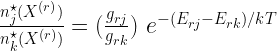
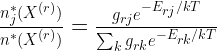
- For example,

In his book, Spitzer defines something called “Equivalent Thermodynamic Equilibrium” or “ETE”. In ETE,  gives the “equivalent” density in state j. The true (observed) value is
  . He then defines the ratio of the true density to the ETE density to be
 .
.
This quantity approaches 1 when collisions dominate over ionization and recombination. For LTE,  for all levels. The level population is then given by the Boltzmann equation:
 ,
,
where  and
and  are the energy and statistical weight (degeneracy) of level j, ionization state r. The exponential term is called the “Boltzmann factor”‘ and determines the relative probability for a state.
The term “Maxwellian” describes the velocity distribution of a 3-D gas. “Maxwell-Boltzmann” is a special case of the Boltzmann distribution for velocities.
Using our definition of b and dropping the “r” designation,

Where  is the frequency of the radiative transition from k to j. We will use the convention that
  , such that
  .
.
To find the fraction of atoms of species  excited to level j, define:

as the particle density of in all states. Then
Define  , the “partition function” for species , to be the denominator of the RHS of the above equation. Then we can write, more simply:
to be the fraction of particles that are in state j. By computing this for all j we now know the distribution of level populations for ETE.
The Saha Equation
(updated for 2013)
How do we deal with the distribution over different states of ionization r? In thermodynamic equilibrium, the Saha equation gives:
 ,
,
where and  are the partition functions as discussed in the previous section. The partition function for electrons is given by

For a derivation of this, see pages 103-104 of this handout from Bowers and Deeming.
If and are approximated by the first terms in their sums (i.e. if the ground state dominates their level populations), then
 ,
,
where  is the energy required to ionize from the ground (j = 1) level. Ultimately, this is just a function of and
  . This assumes that the only relevant ionization process is via thermal collision (i.e. shocks, strong ionizing sources, etc. are ignored).
Important Properties of Local Thermodynamic Equilibrium
(updated for 2013)
For actual local thermodynamic equilbrium (not ETE), the following are important to keep in mind:
- Detailed balance: transition rate from j to k = rate from k to j (i.e. no net change in particle distribution)
- LTE is equivalent to ETE when or

- LTE is only an approximation, good under specific conditions.
- Radiation intensity produced is not blackbody illumination as you’d want for true thermodynamic equilibrium.
- Radiation is usually much weaker than the Planck function, which means not all levels are populated.
- LTE assumption does not mean the Saha equation is applicable since radiative processes (not collisions) dominate in many ISM cases where LTE is applicable.
Definitions of Temperature
(updated for 2013)
The term “temperature” describes several different quantities in the ISM, and in observational astronomy. Only under idealized conditions (i.e. thermodynamic equilibrium, the Rayleigh Jeans regime, etc.) are (some of) these temperatures equivalent. For example, in stellar interiors, where the plasma is very well-coupled, a single “temperature” defines each of the following: the velocity distribution, the ionization distribution, the spectrum, and the level populations. In the ISM each of these can be characterized by a different “temperature!”
Brightness Temperature
 the temperature of a blackbody that reproduces a given flux density at a specific frequency, such that
Note: units for  are
are  .
.
This is a fundamental concept in radio astronomy. Note that the above definition assumes that the index of refraction in the medium is exactly 1.
Effective Temperature
 (also called
  , the radiation temperature) is defined by
 ,
,
which is the integrated intensity of a blackbody of temperature .  is the Stefan-Boltzmann constant.
Color Temperature
 is defined by the slope (in log-log space) of an SED. Thus is the temperature of a blackbody that has the same ratio of fluxes at two wavelengths as a given measurement. Note that
  for a perfect blackbody.
Kinetic Temperature
 is the temperature that a particle of gas would have if its Maxwell-Boltzmann velocity distribution reproduced the width of a given line profile. It characterizes the random velocity of particles. For a purely thermal gas, the line profile is given by
 ,
,
where  in frequency units, or
 in velocity units.
In the “hot” ISM is characteristic, but when  (where
  are the Doppler full widths at half-maxima [FWHM]) then does not represent the random velocity distribution. Examples include regions dominated by turbulence.
can be different for neutrals, ions, and electrons because each can have a different Maxwellian distribution. For electrons,  , the electron temperature.
Ionization Temperature
 is the temperature which, when plugged into the Saha equation, gives the observed ratio of ionization states.
Excitation Temperature
 is the temperature which, when plugged into the Boltzmann distribution, gives the observed ratio of two energy states. Thus it is defined by
 .
.
Note that in stellar interiors,  . In this room,
  , but
, but  .
.
Spin Temperature
 is a special case of for spin-flip transitions. We’ll return to this when we discuss the important 21-cm line of neutral hydrogen.
Bolometric temperature
 is the temperature of a blackbody having the same mean frequency as the observed continuum spectrum. For a blackbody,
  . This is a useful quantity for young stellar objects (YSOs), which are often heavily obscured in the optical and have infrared excesses due to the presence of a circumstellar disk.
Antenna temperature
 is a directly measured quantity (commonly used in radio astronomy) that incorporates radiative transfer and possible losses between the source emitting the radiation and the detector. In the simplest case,
 ,
,
where  is the telescope efficiency (a numerical factor from 0 to 1) and
  is the optical depth.
Excitation Processes: Collisions
(updated for 2013)
Collisional coupling means that the gas can be treated in the fluid approximation, i.e. we can treat the system on a macrophysical level.
Collisions are of key importance in the ISM:
- cause most of the excitation
- can cause recombinations (electron + ion)
- lead to chemical reactions
Three types of collisions
- Coulomb force-dominated (
 potential): electron-ion, electron-electron, ion-ion
- Ion-neutral: induced dipole in neutral atom leads to
 potential; e.g. electron-neutral scattering
- neutral-neutral: van der Waals forces ->
 potential; very low cross-section
We will discuss (3) and (2) below; for ion-electron and ion-ion collisions, see Draine Ch. 2.
In general, we will parametrize the interaction rate between two bodies A and B as follows:
In this equation,  is the collision rate coefficient in
  , where
  is the velocity-dependent cross section and
  is the particle velocity distribution, i.e. the probability that the relative speed between A and B is v. For the Maxwellian velocity distribution,
 ,
,
where  is the reduced mass. The center of mass energy is
  , and the distribution can just as well be written in terms of the energy distribution of particles,
  . Since
  , we can rewrite the collision rate coefficient in terms of energy as
 .
.
These collision coefficients can occasionally be calculated analytically (via classical or quantum mechanics), and can in other situations be measured in the lab. The collision coefficients often depend on temperature. For practical purposes, many databases tabulate collision rates for different molecules and temperatures (e.g., the LAMBDA databsase).
For more details, see Draine, Chapter 2. In particular, he discusses 3-body collisions relevant at high densities.
Neutral-Neutral Interactions
(updated for 2013)
Short range forces involving “neutral” particles (neutral-ion, neutral-neutral) are inherently quantum-mechanical. Neutral-neutral interactions are very weak until electron clouds overlap ( cm). We can therefore treat these particles as hard spheres. The collisional cross section for two species is a circle of radius r1 + r2, since that is the closest two particles can get without touching.

What does that collision rate imply? Consider the mean free path:

This is about 100 AU in typical ISM conditions ( )
)
In gas at temperature T, the mean particle velocity is given by the 3-d kinetic energy:  , or
, or
 , where
  is the mass of the neutral particle. The mean free path and velocity allows us to define a collision timescale:
 .
.
- For (n,T) = (
 ), the collision time is 500 years
- For (n,T) = (
 ), the collision time is 1.7 months
- For (n,T) = (
 ), the collision time is 45 years
So we see that density matters much more than temperature in determining the frequency of neutral-neutral collisions.
Ion-Neutral Reactions
(updated for 2013)
In Ion-Neutral reactions, the neutral atom is polarized by the electric field of the ion, so that interaction potential is
 ,
,
where  is the electric field due to the charged particle,
  is the induced dipole moment in the neutral particle (determined by quantum mechanics), and is the polarizability, which defines
  for a neutral atom in a uniform static electric field. See Draine, section 2.4 for more details.
This interaction can take strong or weak forms. We distinguish between the two cases by considering b, the impact parameter. Recall that the reduced mass of a 2-body system is  In the weak regime, the interaction energy is much smaller than the kinetic energy of the reduced mass:
 .
.
In the strong regime, the opposite holds:
 .
.
The spatial scale which separates these two regimes corresponds to  , the critical impact parameter. Setting the two sides equal, we see that
The effective cross section for ion-neutral interactions is

Deriving an interaction rate is tricker than for neutral-neutral collisions because  in general. So, let’s leave out an explicit n and calculate a rate coefficient k instead, in
  .
.
 (although really
  , so k is largely independent of v). Combining with the equation above, we get the ion-neutral scattering rate coefficient

As an example, for  interactions we get
  . This is about the rate for most ion-neutral exothermic reactions. This gives us
 .
.
So, if  , the average time between collisions is 16 years. Recall that, for neutral-neutral collisions in the diffuse ISM, we had
  years. Ion-neutral collisions are much more frequent in most parts of the ISM due to the larger interaction cross section.
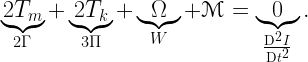
The Virial Theorem
(Transcribed by Bence Beky). See also these slides from lecture
See Draine pp 395-396 and appendix J for more details.
The Virial Theorem provides insight about how a volume of gas subject to many forces will evolve. Lets start with virial equilibrium. For a surface S,

see Spitzer pp.~217–218. Here I is the moment of inertia:

 is the bulk kinetic energy of the fluid (macroscopic kinetic energy):
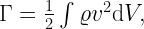
 is
is  of the random kinetic energy of thermal particles (molecular motion), or
  of random kinetic energy of relativistic particles (microscopic kinetic energy):

 is the magnetic energy within S:

and W is the total gravitational energy of the system if masses outside S don’t contribute to the potential:

Among all these terms, the most used ones are ,  and
and  . But most often the equation is just quoted as
 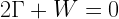 . Note that the virial theorem always holds, inapplicability is only a problem when important terms are omitted.
This kind of simple analysis is often used to determine how bound a system is, and predict its future, e.g. collapse, expansion or evaporation. Specific examples will show up later in the course, including instability analyses.
The virial theorem as Chandrasekhar and Fermi formulated it in 1953 is the following:
This uses a different notation but expresses the same idea, which is very useful in terms of the ISM.
Radiative Transfer
The specific intensity of a radiation field is defined as the energy rate density with respect to frequency, cross sectional area, solid angle and time:
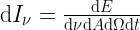
![[\mathrm dI_\nu] = 1 \;\mathrm{erg} \; \mathrm {Hz}^{-1} \; \mathrm {cm}^{-2} \; \mathrm {sr}^{-1} \; \mathrm s ^{-1}](https://s0.wp.com/latex.php?latex=%5B%5Cmathrm+dI_%5Cnu%5D+%3D+1+%5C%3B%5Cmathrm%7Berg%7D+%5C%3B+%5Cmathrm+%7BHz%7D%5E%7B-1%7D+%5C%3B+%5Cmathrm+%7Bcm%7D%5E%7B-2%7D+%5C%3B+%5Cmathrm+%7Bsr%7D%5E%7B-1%7D+%5C%3B+%5Cmathrm+s+%5E%7B-1%7D+&bg=FFFFFF&fg=000000&s=2&c=20201002)
in cgs units. It is important to note that specific intensity does not change during the propagation of a ray, no matter what its geometry is, unless there is extinction or emission in the path.
Specific intensity is a function of position, frequency, direction and time. Integrating over all directions, we get the specific flux density, which is a function of position, frequency and time:

![[F_\nu] = 1 \;\mathrm{erg} \; \mathrm {Hz}^{-1} \; \mathrm {cm}^{-2} \; \mathrm s ^{-1}](https://s0.wp.com/latex.php?latex=%5BF_%5Cnu%5D+%3D+1+%5C%3B%5Cmathrm%7Berg%7D+%5C%3B+%5Cmathrm+%7BHz%7D%5E%7B-1%7D+%5C%3B+%5Cmathrm+%7Bcm%7D%5E%7B-2%7D+%5C%3B+%5Cmathrm+s+%5E%7B-1%7D&bg=FFFFFF&fg=000000&s=2&c=20201002)
where  is usually assumed to be zero.
A conventional unit of specific flux density, especially in radioastronomy, is jansky, named after the American radio astronomer Karl Guthe Jansky:

The specific energy density of a radiation field is
![[u_\nu] = 1 \;\mathrm{erg} \; \mathrm {Hz}^{-1} \; \mathrm {cm}^{-3}](https://s0.wp.com/latex.php?latex=%5Bu_%5Cnu%5D+%3D+1+%5C%3B%5Cmathrm%7Berg%7D+%5C%3B+%5Cmathrm+%7BHz%7D%5E%7B-1%7D+%5C%3B+%5Cmathrm+%7Bcm%7D%5E%7B-3%7D&bg=FFFFFF&fg=000000&s=2&c=20201002)
The mean specific intensity is the specific intensity at a given position and time averaged over all directions:

![[J_\nu] = 1 \;\mathrm{erg} \; \mathrm {Hz}^{-1} \; \mathrm {cm}^{-2} \; \mathrm {s}^{-1}](https://s0.wp.com/latex.php?latex=%5BJ_%5Cnu%5D+%3D+1+%5C%3B%5Cmathrm%7Berg%7D+%5C%3B+%5Cmathrm+%7BHz%7D%5E%7B-1%7D+%5C%3B+%5Cmathrm+%7Bcm%7D%5E%7B-2%7D+%5C%3B+%5Cmathrm+%7Bs%7D%5E%7B-1%7D&bg=FFFFFF&fg=000000&s=2&c=20201002)
The above “specific” quantities all have their frequency integrated counterparts: intensity, flux density, energy density and mean intensity.
The emission and absorption coefficients  and
and  are defined as the coefficients in the differential equations governing the change of intensity in a ray transversing some medium:
The emissivity  and opacity
  are defined by

To find the integral equation determining the specific intensity as a function of path, we define the source function  and the differential optical depth
  by
by
 ;
; 
It is left as an exercise to the reader that these lead to the Radiative Transfer Equation

If the source function is constant in a medium, then the two limiting cases are
- optically thin
 :
: 
- optically thick
 :
: 
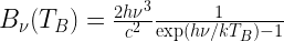
The Planck function, named after the German physicist Max Karl Ernst Ludwig Planck, is

Planck’s law says that a black body, that is, an optically thick object in thermal equilibrium, will emit radiation of specific intensity given by the Planck function, also known as the blackbody function. Any radiation with this specific intensity is called blackbody radiation. A similar concept is thermal emission, which in fact is defined as  , therefore only implies blackbody radiation if the emitting medium is optically thick. Note that in case of thermal emission, one can substitute the definition of source function to write
  , which is known as Kirchoff’s law.
The brightness temperature  of a radiation of specific intensity
  at a given frequency
  is defined as the temperature that a black body would have to have in order to have the same specific intensity:

There are two asymptotic approximations of the blackbody radiation: if  , that is, small frequency or high temperature, we have the Rayleigh–Jeans approximation for the specific intensity:

This is valid in most areas of radio astronomy, except for example some cases of thermal dust emission.
In the other limit, where  , that is, large frequency or low temperature, we have the Wien approximation, named after the German physicist Wilhelm Carl Werner Otto Fritz Franz Wien who derived it in 1983:

The brightness temperature  of a radiation of specific intensity at a given frequency is defined as the temperature that a black body would have to have in order to have the same specific intensity:

Now assume the background radiation of brightness temperature  traverses a medium of temperature T, source function
  , and optical depth
  . In the Rayleigh–Jeans regime
  , therefore the differential and integral forms of the radiative transfer equation become

where is the brightness temperature of the radiation leaving the medium.
This can be applied to dust emission observations assuming an “emissivity-modified” blackbody radiation. Then the contribution of particles of a given linear size a is
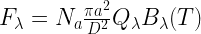
where  is the number of such particles,
  is the distace to the observer, and
  is the emissivity. Recall that the blackbody intensity with respect to wavelength is

We refer the reader to Hilebrand 1983.
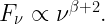
It turns out that the emissivity in far infrared follows a power law:

 for blackbody
 for amorphous lattice-layer materials
 for metals and crystalline dielectrics}
The observed flux will be
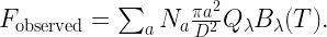
The same emission can be a result of different values of T, Q, and N.
To determine the total mass of dust, we write

where  is an average weighted appropriately.
If  , then emission essentially depends on grain surface area, and we can write

Hildebrand 1983 gives us an empirical formula for dust opacity, implicitly assuming a gas-to-dust ratio of 100, which can be extended with the power law described above to arrive at

A typical modern value for interstellar dust is  , but it is highly disputed. It can be determined based on the SED slope in the Rayleigh–Jeans regime, where
ISM of the Milky Way
The ISM in the Milky way can be divided into cold stuff and hot stuff. Cold stuff are dust and gas. Katherine will talk briefly about the importance of cooling via CO emission. Hot stuff will be discussed by Ragnhild and Vicente (also see Spitzer 1958), and Tanmoy already talked about supernovae. Suggested reading is Chapters 5 and 19 of Draine. In particular, if you ever need a reference of term symbols (uppercase Greek letters with subscripts and superscripts), see page 39.
Cold ISM
The molecular gas is mostly composed of  molecules. This, however, rarely can be observed directly: it has no dipole moment, therefore no rovibrational energy levels. (As exceptions, UV absorption lines can be observed in hot gas, vibrational lines can be observed in shocked ISM, and NIR lines can be observed in “cold” hot ISM.) Instead of observing hydrogen lines, trace species are used as proxies to infer hydrogen density. The choice of preferred trace species depends on their abundance. To quantify this, we define the critical density as

where A is the Einstein coefficient and  is the collision rate for a given transition. This of course will depend on temperature, as the collision rate is the product of the temperature-independent collisional cross section
  and the temperature-dependent particle velocity v. For a detailed explanation of critical density, see pp.~81–87 of Spitzer, and Chapter 19 of Draine.
Typically assumed values are 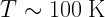 ,
,  ,
,  ,
,  . The Einstein coefficient for the
  transition of CO is
  , yielding a critical density of
 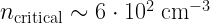 . Spitzer gives us fiducial values for critical densities around
  :
:
- CO,
 ,
,  mm,
mm,  ,
, 
 ,
, 
 mm,
mm,  ,
, 
- CS,
 ,
,  mm,
mm,  ,
, 
- HCN, ,
 mm,
mm,  ,
, 
In practice, the following tracers are used for cold clouds in the range of  :
:
- Low density (n=10 cm^-3): 12CO
- Dark Cloud (n=300): 13CO, OH
- Dense Core (n=10^3): C18O, CS
- Dense Core (n=5 * 10^3): NH3, N2H+, CS
- Very Dense (n=10^8): OH Masers
- Very Very Dense (n=10^10): H20 masers
See handout on dense core multi-line half power contours from Myers 1991, and note that sizes do not proceed as critical densities would suggest.
As a reminder, electronic energy levels are much further apart, resulting in higher frequency transition lines. Vibrational levels are a few orders of magnitude more tightly spaced, then rotational energy levels are even closer. Here we give a brief overview of rotational line structure, see Chapter 5.1.5 of \cite{draine:2010} for more details.
Quantum mechanically, a diatomic molecule has energy levels identified by  with energy
  (which would have
  instead in the quasiclassical theory). Here
  is the moment of inertia,
  is the distance between the atoms, and
  is their reduced mass.
  is the rotation constant. The
  index signifies that these values are valid for a given vibrational state only. Therefore the transition energy between the states J-1 and J is

In case of  O,
O, 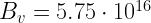 in some mysterious units. For the transition,
 , corresponding to
  , or
, or  . The
. The  and
and  transitions have twice and three times higher energy differences, respectively.
We can estimate which transition gives maximum emission (in terms of number of photons) at a given temperature:

- The SMA and ALMA are sensitive to J=4-7
- KAO and Sophia are sensitive to J=20-40
Note that  at 2.6 mm is more visible from Earth than
  due to atmospheric extinction.
Collisional Excitation
In LTE, the transition rates for a collisional  transition are


where  is the rate coefficent for the transition, is the collisional cross section and v is the particle velocity.
In case of Maxwellian velocity distribution, we have
where is the reduced mass. For neutral-neutral state transitions, is typically  , and for an ionizing transition,
  .
.
In equilibrium, we have


where  is the critical density. When
  , collisions dominate over spontaneous emission, resulting in
However, in case of  , spontaneous emission dominates decay, so each collisionally excitation results in an emission:

In case of optically thin emission,

where  is the apparent solid angle of the source. Then


Recombination of Ions with Electrons
For more details, see Draine Chapter 14.
In HII regions, most recombination happens radiatively: 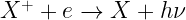 .
.
An electron with kinetic energy “E” can recombine to any level of hydrogen. The energy of the photon emitted is then given by  , where
  is the binding energy of quantum state nl.
There are two extreme cases in recombination (see Baker and Menzel 1938):
- Case A: The medium is opcially thin to ionizing radiation. Appropriate in shock-heated regions (
 ) where density is very low.
- Case B: Optically thick to ionizing radiation. When a atom recombines to the n=1 state, the emitted lyman photon is immediately reabsorbed, so that recombinations to n=1 does not change the ionization state. This is called the “on the spot” approximation
Optical tracers of recombination:  and other lines
Radio: Radio recombination lines (see Draine 10.7). Rydberg States are recombinations to very high (n>100) hydrogen energy levels. Spontaneous decay gives
![\nu_{n\alpha} = \frac{2n+1}{[n(n+1)]^2} \frac{I_H}{h} \sim 6.479 \big(\frac{100.5}{n+0.5}\big)^3 {\rm GHz}](https://s0.wp.com/latex.php?latex=%5Cnu_%7Bn%5Calpha%7D+%3D+%5Cfrac%7B2n%2B1%7D%7B%5Bn%28n%2B1%29%5D%5E2%7D+%5Cfrac%7BI_H%7D%7Bh%7D+%5Csim+6.479+%5Cbig%28%5Cfrac%7B100.5%7D%7Bn%2B0.5%7D%5Cbig%29%5E3+%7B%5Crm+GHz%7D&bg=FFFFFF&fg=000000&s=2&c=20201002)
A popular line is  . This is often observed because its proximity to the 1420 MHz line of HI.
Radio recombination lines often involve masing.
Star Formation in Molecular Clouds
Topics to be covered include:
- The Jeans Mass
- Free Fall Time
- Virial Theorem
- Instabilities
- Magnetic Fields
- Non-Isolated Systems
- “Turbulence”
An overview of the steps of star formation.
Basic properties of a GMC
Mass: 
Lifetime: Uncertain. Probably 10 Myr (maybe as long as 100 Myr). “Lifetime” is not easily defined or inferred, since clouds are constantly fragmenting, exchanging mass with their surroundings, etc.
We roughly describe the hierarchy and fragmentation of clouds via the following terms:
- Clump. 10-100
 . 1pc. The progenitor of stellar clusters
- Core. 1-10 . 0.1 pc. The progenitor of individual stars, and small stellar systems.
- Star. The end-product of fragmentation and collapse. 1 .
Note that, across these scales, density increases by tens of orders of magnitude:

\begin{figure}
\includegraphics[width=4in]{fig_030811_01}
\caption{Schematic of how a GMC fragments into clumps, cores, and stars}
\end{figure}
The Jeans Mass
For further details, see Draine ch 41.
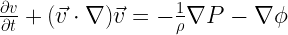
Let’s analyze the stability of a sphere of gas, where thermal pressure is balanced by self-gravity.
Start with the basic hydro equations (conservation of mass, momentum, and Poisson’s equation for the gravitational potential):


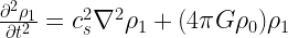
Consider an equilibrium solution  such that time derivatives are zero. Let’s perturb that solution slightly, and analyze when that perturbation grows unstably.
 .
.
The linear hydro equations, to first order in the perturbations, are


Lets restrict our attention to an isothermal gas, so the equation of state is  , where
  is the isothermal sound speed. Then, the momentum becomes

Jeans took these equations and added:
- Uniform density to start with (
 )
)
- Stationary gas (
 )
)
- Gradient-free equilibrium potential
 )
)
Then, the solution becomes (after taking  the momentum equation)
Now consider plane wave perturbations


Define 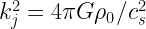 , so
, so

 is reall IFF
  . Otherwise, is imaginary, and there is exponential growth of the instability. This then leads to a Jeans Length:

Gas is “Jeans Unstable” when  . Exponentially growing perturbations will cause the gas to fragment into parcels of size
  .
.
Converting the Jeans length into a radius (assuming a sphere) yields

This defines a “preferred mass” for substructures within a cloud.
Let’s plug in values for a dense core:  . This yields
  . If we instead plug in numbers appropriate for the mean conditions in a GMC,
  , we get
  .
.
Note that, once gravitaional collapse and heating set in, our isothermal sphere assumptions are no longer valid.
Collapse Timescale
For large scales, the growth time for the Jeans instability is

For  , this is about 0.7 Myr. Compared to a “free fall time” (collapse timescale for a pressure-less gas),

For  this is 1.4 Myr — slightly longer than growth time.
The Jeans Swindle
There is a sinister flaw in Jean’s analysis. Assuming  implies that
  . The only way to satisfy this everywhere is for
  . However, more rigorous analysis verifies that Jean’s approach still yields approximately correct results.
More Realistic Treatment
The Bonnor Ebert Sphere is the “largest mass an isothermal gas sphere can have in a \textbf{pressurized medium} while staying in hydrostatic equilibrium.
Numerical Star Formation Simulations
(Notes from Guest Lecture by Stella Offner)
We start by writing down the conservation laws for mass, momentum and energy, each in the form of “rate of change of conserved quantity + flux = source density”:


Also, the Poission equation for gravity is
The initial conditions are determined by T,  , and bulk
  , which further determine the total mass, total angular momentum, turbulence and other global properties.
Grid-based codes
One type of star formation simulations is grid-based. Many of these feature adaptive mash refinement, increasing spatial resolution in areas where parameters vary on smaller scales. Examples of such codes are Orion, Ramses, Athena, Zeus and Enzo.
This algorithm stores  and
and  values at nodes indexed by j. The values at time step n+1 are calculated from those at time step n by discretized versions of the conservation equations. For instance, a discretized mass equation can be written as
First, a homogeneous grid is created, with resolution satisfying the Truelove condition, also called as the Jeans condition:
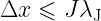
where the empirical value for the Jeans number J is  . Then the simulation is carried on, repartitioning a square by adding nodes if deemed necessary based on the spatial variation of or . The timestep is global, but it can also be adaptively changed, as long as it satisfies the Courant condition

ensuring that gas particles do not move more than half a cell in one time step.
Particle-Based Codes
The other family of codes is particle-based, also referred to as smooth particle hydrodynamics codes. Here individual pointlike particles are traced. Examples codes are Gadget, Gasoline and Hydra.
To solve the equations, density has to be smoothed with a smoothing length h that has to be larger than the characteristic distance between the particles. Usually we want approximately twenty particles within the smoothing radius. The formula for smoothing is

where an example of the smoothing kernel is

where  .
.
The Lagrangian of the system is
 .
.
The Euler–Lagrange equations governing the motion of the particles are

It turns out that solving these equations leads to
 ,
,
where  is an viscosity term added artificially for more accurate modeling of transient behavior. The nature of the simulation requires that particles are stored in a data structure that facilitates easy search based on their position, for example a tree. As particles move, this structure needs to be updated.
The Jeans condition for these kind of simulations is that

where  is the minimum resolved fragmentation mass, equal to the typical total mass within smoothing length from any particle.
Comparison
The advantages of the grid-based codes is that they are
- accurate for simulating shocks,
- more stable at instabilities.
Their disadvantages are that
- grid orientation may cause directional artifacts,
- grid imprinting might appear at the edges.
Also, they are more likely to break if there’s a bug in the code. On the other hand, particle-based codes have the advantages of being
- inherently Lagrangian,
- inherently Galilei invariant, that is, describing convection and flows well,
- accurate with gravity,
- good with general geometries.
At the same time, they suffer from
- resolution problems in low density regions,
- the need for an artificial viscosity term,
- the need for post processing to extract information on density and momentum distribution,
- statistical noise.
See slides for the effect of too large J for a grid-based simulation, too small h for a particle-based simulation, for examples involving shock fronts, Kelvin–Helmholtz instability and Rayleigh–Taylor instability, and star formation. Note that the simulated IMF matches theory and observations within an order of magnitude, but this is very sensitive to the initial temperature of the molecular cloud.
Some thoughts on Jeans scales
Recall the equation for the Jeans Mass:
In common units, this is

This raises a question — what jeans mass do we choose if a gas cloud is hierarchical, with many different densities and temperatures? This motivates the idea of turbulent fragmentation, wherein a collapsing cloud fragments at several scales as it collapses. We will return to this
Also recall that the Jeans growth timescale for structures much larger than the Jeans size is

for 
Compare this to the pressureless freefall time:

From which we see

The Jeans growth time is about 1/2 the free-fall time
Finally, compare this to the crossing time in a region with  . The sound speed is
  , which is 0.27 km/s for molecular hydrogen, and .08 km/s for 13CO.
However, note that the observed linewidth in 13CO for such regions is of the order 1 km/s. Clearly, non-thermal energies dominate the motion of gas in the ISM.
Recall that the jeans length is 
Plugging in the thermal H2 sound speed yields  . The crossing time for CO gas moving at 1 km/s is thus 1Myr in this region.
So, in a cloud with  and
and  , the Jeans growth time, free fall time, and crossing time are all comparable.
There is a problem with our derivation, though! We assumed the relevant sound speed that sets the Jeans length is the thermal hydrogen sound speed. However, these clouds are not supported thermally, as the non-thermal, turbulent velocity dispersion dominates the observed linewidths. This suggests we use and equivalent Jeans length where we replace the sound speed by the turbulent linewidth.
This is often done in the literature, but its sketchy. Using turbulent linewidths in a virial analysis assumes that turbulence acts like thermal motion — i.e., it provides an isotropic pressure. This may not be the case, as turbulent motions can be partially ordered in a way that provides little support against gravity.
The question of how a cloud behaves when it is not thermally supported leads to a discussion of Larsons Laws (JC 2013)
Larsons Legacy
see these slides
Stellar Winds in Star Forming Regions
Guest Lecture by Hector Arce. See this post for notes. See also this movie
Introduction to shocks
Shocks occur when density perturbations are driven through a medium at a speed greater than the sound speed in that medium. When that happens, sound waves cannot propagate and dissipate these perturbations. Overdense material then piles up at a shock front
Collisions in the shock front will alter the density, temeprature, and pressure of the gas. The relevant size scale over which this happens (i.e., the size of the shock front) is the size scale over which particles communicate with each other via collisions:
 . If
. If 

A shock
An excellent reference offering a three-page summary of important shock basics (including jump conditions) is available in this copy of a handout from Jonathan Williams ISM class at the IfA in Hawaii.
Shock De-Jargonification
See this handout and this list of examples.
Shock(ing facts about) viscosity
A perfect shock is a discontinuity, but real shocks are smoothed out by viscosity. Viscosiity is the resistance of a fluid to deformation (it is the equivalent of friction in a fluid)
Inviscid or ideal fluids have zero viscosity. Colder gasses are less viscious, because collisions are less frequent.
Simulations include numerical viscosity by accident — these are the result of computational approximations / discretization that violate Eulers equations and lead to a momentum flow that acts like true viscosity. However, the behavior of numerical viscosity can be unrealistic and of inappropriate magnitude
True shocks are a few mean free paths thick, which is typically less than the resolution of simulations. Thus, simulations also add artificial viscosity to smooth out and resolve shock fronts.
Rankine Hugoniot Jump Conditions
This section is based on the 2013 Wikipedia entry for “Rankine-Hugoniot Conditions,” archived as a PDF here.
The Jump conditions describe how properties of a gas change on either side of a shock front. They are obtained by integrating the Euler Equations over the shock front. As a reminder, the mass, momentum, and energy equations in 1 dimension are
Where  is the fluid specific energy, and
  is the internal (non-kinetic) specific energy.
We supplement these equations with an equation of state. For a adiabatic shocks (a bad term, but describes shocks where radiative losses are small), the equation of state is 
Generally, what a jump condition is a condition that holds at a near-discontinuity. It ignores the details about how a quantity changes across the discontinuity, and instead describes the quantity on either side.
The general conservation law for some quantity w is

A shock is a jump in w at some point  . We call x1 the point just upstream of the shock, and x2 the point just downstream

A schematic defining the notation for the shock jump conditions
Integrating the conservation equation over the shock,


This holds because  in the frame moving with the shock
Let  when
when

and in the limit 
Where 

The upstream and downstream speeds are constrained via

Moving away from the generic w formalism and to the Euler equations, we find
These are the Rankine Hugoniot conditions for the Euler Equations.
In going to a frame co-moving with the shock (i.e. v = S – u), one can show that

where c1 is the upstream sound speed 
For a stationary shock, S = 0 and the 1D Euler equations become


After more substitution and defining  ,
,
For strong (adiabatic) shocks and an monatomic gas ( ),
),

Introduction to Instabilities
See this handout
Rayleigh-Taylor Instability
The Rayleigh-Taylor instability occurs when a more dense fluid rests on top of a less dense fluid, in the presence of a gravitational potential  (though note that accelerations mimic gravity, so many driven jets, etc exhibit the RT instability without gravity)

Notation for the RT instability
To derive the instability, we will solve the momentum and continuity equations while satisfying boundary conditions at the a/b interface
The momentum equation is
![\rho \frac{DV}{Dt} = \rho [ \frac{dv}{dt} + v \cdot \nabla v] = - \nabla P - \frac1{8 \pi} \nabla B^2 + \frac1{4 \pi} B \cdot \nabla B - \rho \nabla \phi](https://s0.wp.com/latex.php?latex=%5Crho+%5Cfrac%7BDV%7D%7BDt%7D+%3D+%5Crho+%5B+%5Cfrac%7Bdv%7D%7Bdt%7D+%2B+v+%5Ccdot+%5Cnabla+v%5D+%3D+-+%5Cnabla+P+-+%5Cfrac1%7B8+%5Cpi%7D+%5Cnabla+B%5E2+%2B+%5Cfrac1%7B4+%5Cpi%7D+B+%5Ccdot+%5Cnabla+B+-+%5Crho+%5Cnabla+%5Cphi&bg=FFFFFF&fg=000000&s=2&c=20201002)
The continuity equation is
To satisfy the continuity equation, we introduce a velocity potential

The density is constant (in time) above and below the interface, so the continuity equation implies 
A solution satisfying  for very large Z is
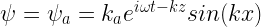 above
above below
below
Where  is the wave number
Take the real part of  as the physical answer. Let B = 0, and ignore
  in the momentum equation. By integrating the momentum equation over space, we find
which holds separately above and below the interface
The boundary conditions are that  need to be continuous across the interface
We can find the z of the interface,  , by integrating
  over time, so
To first order in
If is continuous across the boundary then must be the same above and below so
 at
at 
This implies that 
Continuity of pressure across the intervace gives
Using the equation for and noting  at z=0 gives
If  then is imaginary, and the instability grows with time
Ionization fronts, HII regions, Stellar Winds, and Disk Structure
Although these 4 objects exist at different scales, their evolutions are coupled. Lets explore this connection
Ionization fronts are caused by stars with large fluxes of ionizing photons. We see them around HII regions. We observe them emission from several ionizaed specias, especially as they recombine and cool
We would like to know how ionization fronts form, expand, and emit. We would also like to know their lifetime, and how different ionization fronts map to different stars in a crowded environment.
The expansion of HII regions is influenced by the time dependent evolution of both the ionization front and the stellar wind with the surrounding medium. Draine 37.2 calculates the expansion of an HII region into a uniform medium
Stellar Winds
We talked about bi-polar flows, but these are a special type of stellar wind. Other winds are less collimated. Different kinds of winds are associated with stars at different evolutionary states:
Pre main sequence stars: T-tauri winds
Main Sequence winds (like the solar wind)
Post-Main Sequence winds / planetary nebulae
Disk Structure
Disks around stars are accretion disks. The structure of a gravitationally bound disk is governed by Keplerian rotation. However, accretion disks have a temperature structure giving rise to thermal forces (plus magnetic/turbulent forces) that can change their internal structure and dynamics
Ionization Fonts
See chapter 20 of Shus Physics of Astrophysics

Note that the mean free path of photons in an ionized gas is much larger than the mean free path in neutral gas:
- Neutral Gas: Cross section for interaction is size of atom, or
 .
.
- Ionized Gas: Interaction is via Thompson scattering, where the cross section is the size of a free electron.

We already discussed the Stromgren radius, which sets the size of an idealized HII region by balancing the stellar ionizing photon flux with the rate at which the ionized volume recombines and thus quenches this flux:
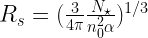
However, this ionized region will have a pressure much higher than the cool, neutral exterior. Thus, HII regions expand over time, and both pressure and ionization fronts are driven into the neutral medium.
Expansion of HII regions
Stage 1
 {graphic}
- Stage begins when a star turns on in a neutral medium
- Rapid expansion of ionization front into static HI cloud
- Very little fluid motion (photons travel much faster than shock waves!)
- This stage ends when the radius approaches the Stromgren radius, and the ionizing photons are quenched by recombinations
Stage 2

- The hot ionized HII region is over-pressured compared to the ambient exterior. This drives a radiative shock
- Sweeps up HI gas into a shell. The ionization front is interior to this shell
- Ends either the star explodes as a supernova, or the radius expands to
 , where recombinations balance ionizing photons and there is pressure balance between the interior and exterior
- Realistically, inhomogeneities in the surrounding medium mean that the HII region will evolve in more complicated ways than this
Stellar Winds
See Lamers and Cassivelli 1999
Wind driving mechanisms:
For cool stars (T = 5000K), winds are driven by the pressure expansion of the hot corona. This is like our own sun
For hot stars (T = 10,000 – 100,000K at the surface), the lack of strong convection inhibits the creation of a hot corona. The temperature at these stars surfaces is not hot enough for particles to escape the gravitational potential. Instead, these stars drive winds directly via radiation pressure. These winds travel at  , and have mass loss rates of
The wind mechanism for pre main sequence stars is debated, but probably involves some interaction between an accretion disk and magnetic field
Disk Structure
The initial evidence for accretion disks around young stars was the SED, which shows an excess of IR emission due to accretion-powered luminosity.
The pioneering paper in this field is Adams, Lada and Shu 1987. See also the review paper by Lada 1999
Young stars were initially divided into 3 evolutionary classes, via the shape of there IR SEDS:
Class 0: SED looks like a single, cold blackbody. Emission is due entirely to a cold core, with no central source

Class 0 YSO
Class I: A large infrared excess, with a rising SED in the infrared. Strong IR excess (compared to the blackbody of a hot, compact central source) is due to a massive disk and outflow

Class I YSO
Class II: A flat IR SED, as the flux of the central source rises, and the disk dissipates

Class III: A faling IR SED. The accretion disk is mostly depleted, and adds only a small infrared excess on top of the SED of the central object.

Class III YSO
Disks in the context of Star and Planet Formation
For excellent references on star and planet formation, see “Protostars and Planets V”, as well as Stahler and Palla’s “The Formation of Stars”
What is a protostar?
I like the wikipedia entry:
“A contracting mass of gass that represents an early stage in the formation of a star before nucleosynthesis has begun”
Since fusion is a negligible energy source in a protostar, its luminosity comes from gravitational contraction. From the virial theorem, half of the gravitational potential energy gain from contraction is converted into kinetic energy, while the other half is radiated away. In other words, for a homogeneous sphere,  .
.
For a 1 solar mass star contracted to  erg.
erg.
What is a planet?
Wikipedia says: “A celestial body moving in an elliptic orbit around a star.” This isn’t quite precise enough — could be an asetroid, KBO, binary star, brown dwarf, etc.
How do planets form?
See this post
Key and Open Questions Regarding the Intergalactic Medium
See also this post
The Kenticutt-Schmidt relation empirically links the surface brightness and star forming rate of galaxies. What is the physical explanation for this? In particular, is there a more prescriptive form or interpretation of the KS relation, that is more astrophysical (and perhaps more accurate at predicting star formation rate)?
Not all galaxies are created equal(ly)
What is the origin of Spiral galaxies? Is the spiral density wave theory of Lin and Shu corre t, or might the GMC perturbation theory of D’Onghia and Hernquist be more apropos? Is the formation of grand design spirals different from that of flocculent spirals?
Where to ellipticals come from? They most likely are the remnants of mergers:
- They they have no ordered rotation. (suggests random mixing)
- Old stars, little or no dust/gas
- Often at the center of clusters
- Always have central Black Holes
“Young” merger galaxies (i.e. before a galaxy has undergone several mergers and formed an elliptical) have extreme star formation rates. SFR can range from 100s to 1000s of stars/year (by comparison, the SFR in the Milky Way is 1 
Significant Variations in the Gas/Dust Ratio and Metallicity
This is true both within galaxies and among galaxies.
How does this affect the K-S relationship?
What are the Kennicutt-Schmidt relations?
See also this post
The “Schmidt Law” is due to Marten Schmidt (1959): “The mean density of a galaxy may determine, as a first aproximation, its present gas content and thus its evolution stage”

Here, n is the volume density.
The “Kennicut Law” is similar to the Schmidt law, but uses the surface density:

Where, typically, q~1.4 (The Schmidt Law above would give q=1.5). Notably q is not 1, which would imply a constant efficiency function.
Some tracers of star formation rate:
- UV flux (from unobscured massive young stars)
- H-alpha flux (also from young stars)
- FIR flux – reprocessed starlight (but– that’s also dependent on gas surface density, so its sketchy to use in the KS law. That doesn’t mean people don’t do it!)
Some tracers of surface density:
- HI
- CO
- HI+CO
- HCN and other tracers that preferentially probe high surface densities. Gao and Solomon 2004 quote

A big issue in using the KS law is how “independent” the tracers of surface density and star formation rate are. Also, the KS relationship extends over many orders of magnitude. Because of this, its unclear whether KS says something important of the conversion of gas into stars, or rather something trivial like “bigger galaxies have more gas, and form more stars”.
The ISM at very high redshift
See this post
Special Topics
See this post


 )
)
 ,
, 


 be the orbiting mass entering and leaving the ring.
  . In the steady state, conservation of energy requires that the energy radiated by an annulus in the the accretion disk be equal to the difference in energy flux between its inner and outer edges. Therefore
  . Equating the two sides gives:
  . The Stefan-Boltzmann relation gives
  .
. . We did not take into account the fact that the star has a finite size which introduces a boundary layer into the disk. A more thorough analysis (e.g. in
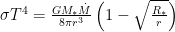
 .
. of a planet accreting planetesimals is of order the Hill radius. Thus we can write
  , where
  is a constant of order unity, and
  is the Hill radius. Furthermore, we note that the mass within this feeding zone can be calculated from the surface density of the disk
  :
: 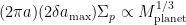
 . We can solve this equation to find that
  .*
.*


 from
from  high-resolution quasar spectra. In addition, we impose the requirements that H I must be reionized by
  and He II by
  and consider estimates of the hardness of the ionizing background from H I-to-He II column density ratios. The derived hydrogen photoionization rate is remarkably flat over the Ly
 , the lack of redshift evolution indicates that star-forming galaxies likely dominate the photoionization rate at
 . Combined with direct measurements of the galaxy UV luminosity function, this requires only a small fraction
  of galactic hydrogen-ionizing photons to escape their source for galaxies to solely account for the entire ionizing background. Under the assumption that the galactic UV emissivity traces the star formation rate, current state-of-the-art observational estimates of the star formation rate density appear to underestimate the total photoionization rate at
 by a factor of
  if extrapolated to arbitrarily high redshift. A theoretical star formation history peaking earlier fits the Ly
 gamma-ray bursts observed by Swift. Quasars suffice to doubly ionize helium by
  ?
? , of hydrogen photoionizing photons for galaxies and quasars?
 by measuring intervening neutral hydrogen absorption. Whereas
  ,
, 
 , the comoving star formation rate density (units of solar masses per year per comoving cubic megaparsec). This means of constraining star formation history is complementary to more direct approaches, for example those using photometric surveys trace the amount of UV light and hence star formation as a function of redshift (see
  Comparison with Prior Results below).
 .
.  of the photoionizing background, which in turn derives from an intrinsic emissivity of astrophysical sources
  . At least some of these sources must be young stars, so that the star formation history
 , where
  is the transmission
 ,
,  , as shown in Fig. 2 below.
 that the authors claim its extrapolation can reionize the Universe in time. Hence, this disagreement with prior work actually appears to be a virtue of the Ly
 , the quasar contribution alone overproduces the photoionizing background. That’s why in Fig. 5 of the text the quasar contribution has been scaled down by factors ranging from 0.1 to 0.35.
 . Since only quasars can contribute the
  eV photons necessary to doubly ionize He II, this requirement roughly fixes the normalization of the quasar luminosity function at the
  of the H I photoionizing background derives from quasar emission. Clearly, there are disagreements yet to be resolved.
 3, and star formation may dominate over quasars at all redshifts considered.
 ) using the IRAC (3.6, 4.5, 5.8, and 8 μm) and MIPS (24, 70, and 160 μm) instruments on board the Spitzer Space Telescope in the Surveying the Agents of a Galaxy’s Evolution (SAGE) survey, these agents being the interstellar medium (ISM) and stars in the LMC. This paper provides an overview of the SAGE Legacy project, including observing strategy, data processing, and initial results. Three key science goals determined the coverage and depth of the survey. The detection of diffuse ISM with column densities
  permits detailed studies of dust processes in the ISM. SAGE’s point-source sensitivity enables a complete census of newly formed stars with masses >3 Msolar that will determine the current star formation rate in the LMC. SAGE’s detection of evolved stars with mass-loss rates >1×10⁻⁸ Msolar yr-1 will quantify the rate at which evolved stars inject mass into the ISM of the LMC. The observing strategy includes two epochs in 2005, separated by 3 months, that both mitigate instrumental artifacts and constrain source variability. The SAGE data are nonproprietary. The data processing includes IRAC and MIPS pipelines and a database for mining the point-source catalogs, which will be released to the community in support of Spitzer proposal cycles 4 and 5. We present initial results on the epoch 1 data for a region near N79 and N83. The MIPS 70 and 160 μm images of the diffuse dust emission of the N79/N83 region reveal a similar distribution to the gas emissions, especially the H I 21 cm emission. The measured point-source sensitivity for the epoch 1 data is consistent with expectations for the survey. The point-source counts are highest for the IRAC 3.6 μm band and decrease dramatically toward longer wavelengths, consistent with the fact that stars dominate the point-source catalogs and the dusty objects detected at the longer wavelengths are rare in comparison. The SAGE epoch 1 point-source catalog has
  sources, and more are anticipated when the epoch 1 and 2 data are combined. Using Milky Way (MW) templates as a guide, we adopt a simplified point-source classification to identify three candidate groups-stars without dust, dusty evolved stars, and young stellar objects-that offer a starting point for this work. We outline a strategy for identifying foreground MW stars, which may comprise as much as 18% of the source list, and background galaxies, which may comprise ~12% of the source list.
 of H or greater. This will allow SAGE to measure the dust-to gas ratio across the ISM and look for variations. This traces the degree of dust-gas mixing in the LMC. One can imagine using this as a proxy for processes like turbulence. Further, by using color ratios and fitting the SED for different grain size distributions, SAGE will be able to study the spatial variation in grain size distribution in the LMC. In particular, SAGE aims to get high-resolution data on
  . The survey should be able to obtain an unbiased, complete census of all such objects throughout the LMC. This should include both massive star formation regions (traced by HII regions) and lower mass star formation regions (traced by Taurus complexes). The two epochs of SAGE data should also allow variability studies for YSOs, looking for objects like
  . This should allow a complete census of evolved stars with appreciable mass loss rates throughout the LMC. The two epochs of SAGE data should also inform studies of variability in mass loss rates, since mass loss processes in evolved stars are also thought to occur on timescales of around a year.
 region corresponding to the LMC was imaged by the telescope in 7 different bands, from the near to far IR. IRAC imaged in the near-IR in the 3.5, 4.5, 5.8 and 8.0
  bands (291 hours) and MIPS in the mid and far IR in the 24, 70 and 160
  means the LMC is nowhere near edge-on, making it much easier to distinguish features. The combination of these features allow resolving features in much greater detail than permitted by imaging more distant galaxies. Further, lines of sight to the LMC are clear of the Small Magellanic Cloud (SMC) and Milky Way (MW). The expectation on the number of substantial clouds per line of sight is small, so if a cloud is detected along a line of sight, it is the only one. Not having to try to separate clouds along the line of sight greatly simplifies the analysis. Further, all clouds are located at approximately the same distance, making comparisons along the line of sight much easier.


 , as compared to a total stellar mass of
  . The authors summarize the work of Whitney et al. (2008) (
 . Whitney et al. note, however, that the UV flux from the LMC gives a higher star formation rate, and that their catalogue of YSOs in the LMC is by no means complete. Meixner et al. note that more recent work presented at the proceedings finds five times as many YSOs using the same color cuts as Whitney et al. Finally, the mass-loss rate of AGB stars is estimated by comparing the 8 μm emission to scaled atmospheric models. The 8 μm excess has been previously correlated to AGB mass-loss rates, and the resulting relation is applied to the entire sample of AGB stars, giving a total mass-loss rate of
  .
., Fig. 5")


")
")
")
")

")
")
")


 is given by
  , where n(t) is the number density of neutral hydrogen at time t, and
  is the cross-section for the Ly-α transition.
  is the redshift at which the photon is being scattered, i.e.
  , where
  of the quasar. Plugging in
  , together with an expression for dl/dz from the cosmology, the total optical depth can be found by integrating over redshift. This again yields a relation between the optical depth and the number density of (neutral) hydrogen.
 model in the paper corresponds to a cosmology where
  .)
.)
 required for forming a central galaxy, so the number of central galaxies is
  , where H is the Heaviside step function. Note this model assumes any one halo will form at most one large star-forming galaxy. The number of satellite galaxies is taken to be
  , where
  and
and  , where
  represents 1-halo clustering (clustering at short scales) and
  represents 2-halo clustering (clustering at long scales).
 . Averaged over all wavebands, the authors find
  , with uncertainty of
  . This result empirically sets a minimum mass scale for the dark matter halo required to form a central, massive star-forming galaxy.


![\frac{d \rho E}{d t} = - \frac{d}{dx} \big[ \rho u (e + 1/2 u^2 + P / \rho) \big]](https://s0.wp.com/latex.php?latex=%5Cfrac%7Bd+%5Crho+E%7D%7Bd+t%7D+%3D+-+%5Cfrac%7Bd%7D%7Bdx%7D+%5Cbig%5B+%5Crho+u+%28e+%2B+1%2F2+u%5E2+%2B+P+%2F+%5Crho%29+%5Cbig%5D+&bg=FFFFFF&fg=000000&s=2&c=20201002)


![S(\rho_2 E_2 - \rho_1 E_1) = \big[ \rho_2 u_2 (e_2 + 1/2 u_2^2 + P_2 / \rho_2) \big] - \big[ \rho_1 u_1 (e_1 + 1/2 u_1^2 + P_1 / \rho_1) \big]](https://s0.wp.com/latex.php?latex=S%28%5Crho_2+E_2+-+%5Crho_1+E_1%29+%3D+%5Cbig%5B+%5Crho_2+u_2+%28e_2+%2B+1%2F2+u_2%5E2+%2B+P_2+%2F+%5Crho_2%29+%5Cbig%5D+-+%5Cbig%5B+%5Crho_1+u_1+%28e_1+%2B+1%2F2+u_1%5E2+%2B+P_1+%2F+%5Crho_1%29+%5Cbig%5D&bg=FFFFFF&fg=000000&s=2&c=20201002)


 above
above below
below


")
 where
where  is the rotational frequency). The necessary conditions for the MRI to develop are the following:


 . So, in an arm, where there is a natural enhancement of the surface density
  , the condensation process is more efficient.
 = Const we have for the local gradient in the angular velocity
  where
where  is the azimuthal average. For instance, for greater than a factor of two overdensity we can actually reverse the direction of the shear. The important point: this allows more time for condensations to grow before they are sheared out.
 .
. ) to be locally unstable.
 ) clumps along the length of the arm are associated with GMCs.